3.3.1: Only one observable (⇐ Only one measurement is permitted )
In this section, we examine the linguistic interpretation $\S$3.1, i.e., "Only one measurement is permitted".
"Only one measurement" implies that "only one observable" and "only one state". That is, we see:
\begin{align}
\qquad
\mbox{[only one measurement]}
\Longrightarrow
\left\{\begin{array}{ll}
\mbox{only one observable (=measuring instrument)}
\\
\\
\mbox{only one state}
\end{array}\right.
\tag{3.10}
\end{align}
$\fbox{Note 3.3}$ Although there may be several opinions, I believe that the standard Copenhagen interpretation ( in physics ) also says "only one measurement is permitted". Thus, some think that this spirit is inherited to quantum language. However, our assertion is reverse,
namely, the Copenhagen standard interpretation is an outcome of the linguistics interpretation. That is, we assert that
${}$ not "$\fbox{Copenhagen interpretation}\Longrightarrow
\fbox{Linguistic interpretation}$"
but "$\fbox{Linguistic interpretation} \Longrightarrow\fbox{Copenhagen interpretation}$"
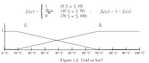
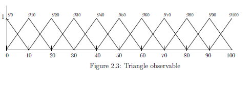
Recall the measurement in Example 2.31 (Cold or hot?) and Example 2.32 (Approximate temperature), and consider the following situation:

$(a):$ There is a cup in which water is filled. Assume that the temperature is $\omega $ °C $(0 {{\; \leqq \;}}\omega {{\; \leqq \;}}100)$. Consider two questions:
${}$ $
\left\{\begin{array}{ll}
\mbox{
"Is this water cold or hot?" (cf. Figure 1.2 below )
}
\\
\\
\mbox{
"How many degrees(°C) is roughly the water?" (cf. Figure 2.3 below )}
\end{array}\right.
$


${}$
$
\left\{\begin{array}{ll}
\mbox{
$(\sharp_1)$:
${\mathsf M}_{L^\infty ( \Omega )} ( {\mathsf O}_{{{{{c}}}}{{{{h}}}}}
{{=}}
(\{{{{{c}}}},{{{{h}}}}\}
, 2^{\{{{{{c}}}},{{{{h}}}}\}}, F_{{{{{c}}}}{{{{h}}}}} ), S_{[\omega]} )$
in
Example 2.31
}
\\
\\
\mbox{
$(\sharp_2)$
:
${\mathsf M}_{L^\infty ( \Omega )}$
$ ({\mathsf O}^{\triangle}
$
$
{{=}}
({\mathbb N}_{10}^{100} ,$
$
2^{{\mathbb N}_{10}^{100} }, G^{\triangle} ),$
$
S_{[\omega]} )
$
in
Example 2.32
}
\end{array}\right.
$

Thus, we have the following problem.
Definition 3.11 [Product measurable space] For each $k =1,2,\ldots,n$, consider a measurable $(X_k , $ ${\cal F}_k )$. The product space $\times_{k=1}^n X_k$ of $X_k$ $(k=1,2,\ldots,n )$ is defined by
\begin{align*} \times_{k=1}^n X_k = \{ (x_1, x_2,\ldots, x_n ) \;|\; x_k \in X_k \;\; (k=1,2,\ldots,n )\} \end{align*}Similarly, define the product $\times_{k=1}^n \Xi_k$ of $\Xi_k ( \in {\cal F}_k )$ $(k=1,2,\ldots,n )$ by
\begin{align*} \times_{k=1}^n \Xi_k = \{ (x_1, x_2,\ldots, x_n ) \;|\; x_k \in \Xi_k \;\; (k=1,2,\ldots,n )\} \end{align*}Furthermore, the $\sigma$-{{field}} $\boxtimes_{k=1}^n{\cal F}_k$ on the {product space} $\times_{k=1}^n X_k$ is defined by
| ${}:$ | $\boxtimes_{k=1}^n{\cal F}_k$ is the smallest field including $ \{ \times_{k=1}^n \Xi_k \;|\; \Xi_k \in {\cal F}_k \;\; (k=1,2,\ldots,n ) \}$ |
$({}\times_{k=1}^n X_k , \boxtimes_{k=1}^n{\cal F}_k)$ is called the product measurable space. Also, in the case that $(X,{\cal F})=(X_k,{\cal F}_k)$ $(k=1,2,\ldots,n)$, the product space $\times_{k=1}^n X_k$ is denoted by $X^n$, and the product measurable space $({}\times_{k=1}^n X_k ,$ $ \boxtimes_{k=1}^n{\cal F}_k)$ is denoted by $(X^n,{\cal F}^n)$.
Definition 3.12 [Simultaneous observable, simultaneous measurement]Consider the basic structure $[{\mathcal A} \subseteq \overline{\mathcal A} \subseteq B(H)]$. Let $\rho \in {\frak S}^p({\mathcal A}^*)$. For each $k =1,2,\ldots,n$, consider a measurement ${\mathsf M}_{\overline{\mathcal A}}$ $({\mathsf O}_ =(X_k , {\cal F}_k , F_k{}), S_{[\rho]} )$ in $\overline{\mathcal A}$. Let $({}\times_{k=1}^n X_k , \boxtimes_{k=1}^n{\cal F}_k)$ be the product measurable space. An observable $\widehat{\mathsf O}$ $=$ $({}\times_{k\in K } X_k ,$ $ \boxtimes_{k=1}^n{\cal F}_k , $ $\widehat{F}{})$ in $\overline{\mathcal A}$ is called the simultaneous observable of $\{ {\mathsf O}_k \;: \; k=1,2,...,n \}$, if it satisfies the following condition:
\begin{align} & {\widehat F}({}\Xi_1 \times \Xi_2 \times \cdots \times \Xi_{n}{}) = F_1 ({}\Xi_1{}) \cdot F_2 ({}\Xi_2{}) \cdots F_n ({}\Xi_{n}{}) \tag{3.11} \\ & \qquad \qquad ( \;\; \forall \Xi_k \in {\cal F}_k \; (k=1,2,\ldots,n )) \nonumber \end{align}
$\widehat{\mathsf O}$ is also denoted by $ \times_{k=1}^n{\mathsf O}_k$, $\widehat{F}$ $=$ $\times_{k=1}^n{F}_k$. Also, the measurement ${\mathsf M}_{\overline{\mathcal A}} (\times_{k=1}^n{\mathsf O}_k, S_{[\rho]})$ is called the simultaneous measurement Here, it should be noted that
| $\bullet$ | the existence of the simultaneous observable $\times_{k=1}^n {\mathsf O}_k$ is not always guaranteed. |
though it always exists in the case that $\overline{\mathcal A}$ is commutative (this is, $\overline{\mathcal A}=L^\infty (\Omega)$).
In what follows, we shall explain the meaning of "simultaneous observable".

However, according to the linguistic interpretation ($\S$3.1), two measurements ${\mathsf M}_{\overline{\mathcal A}}({\mathsf O}_1,$ $ S_{[\rho]})$ and ${\mathsf M}_{\overline{\mathcal A}}({\mathsf O}_2, S_{[\rho ]})$ can not be taken. That is,
\begin{align*} \mbox{The (b) is impossible} \end{align*} Therefore, combining two observables ${\mathsf O}_1$ and ${\mathsf O}_2$, we construct the simultaneous observable ${\mathsf O}_1\times {\mathsf O}_2$, and take the simultaneous measurement ${\mathsf M}_{\overline{\mathcal A}} ( {\mathsf O}_1 \times {\mathsf O}_2, S_{[\rho]})$ in what follows.| $(c):$ | $ \overset{{}}{\underset{ \rho (\in {\frak S}^p({\mathcal A}^*) ) } {{ \fbox{state}}}} \xrightarrow[]{\qquad \qquad} \overset{{}} { \underset{ {\mathsf O}_1 \times {\mathsf O}_2} {{ \fbox{simultaneous observable }}} } \xrightarrow[ {\mathsf M}_{\overline{\mathcal A}} ( {\mathsf O}_1 \times {\mathsf O}_2, S_{[\rho]})]{} \overset{{}} { \underset{ (x_1,x_2) (\in X_1 \times X_2 )} {{ \fbox{measured value }}} } $ |
Answer 3.13 [The answer to Problem 3.10] Consider the state space $\Omega$ such that $\Omega =$ $ [0,100]$, the closed interval. And consider two observables, that is, [C-H]-observable ${\mathsf O}_{{{{{c}}}}{{{{h}}}}}= (X {{=}} \{ {{{{c}}}} , {{{{h}}}} \}, 2^X, F_{{{{{c}}}}{{{{h}}}}} )$ (in Example 2.31) and triangle observable ${\mathsf O}^{\triangle}= (Y( {{=}} {\mathbb N}_{10}^{100}) , 2^Y, G^{\triangle} )$ (in Example 2.32). Thus, we get the simultaneous observable ${\mathsf O}_{{{{{c}}}}{{{{h}}}}} \times {\mathsf O}^{\triangle}$ $=$ $(\{ {{{{c}}}} , {{{{h}}}} \}\times {\mathbb N}_{10}^{100}, 2^{\{ {{{{c}}}} , {{{{h}}}} \}\times {\mathbb N}_{10}^{100}}, F_{{{{{c}}}}{{{{h}}}}} \times G^{\triangle} )$, and we can take the simultaneous measurement ${\mathsf M}_{L^\infty (\Omega)}({\mathsf O}_{{{{{c}}}}{{{{h}}}}} \times {\mathsf O}^{\triangle}, S_{[\omega]})$. For example, putting $\omega=55$, we see
| $(d):$ | when the simultaneous measurement ${\mathsf M}_{L^\infty (\Omega)}({\mathsf O}_{{{{{c}}}}{{{{h}}}}} \times {\mathsf O}^{\triangle}, S_{[55]})$ is taken, the probability \begin{align} & \mbox{that } \mbox{the measured value } \left[\begin{array}{ll} (\mbox{c}, \mbox{about 50°C}) \\ (\mbox{c}, \mbox{about 60°C}) \\ (\mbox{h}, \mbox{about 50°C}) \\ (\mbox{h}, \mbox{about 60°C}) \end{array}\right] \mbox{is obtained is given by} \left[\begin{array}{ll} 0.125 \\ 0.125 \\ 0.375 \\ 0.375 \end{array}\right] \end{align} |
| $\fbox{Note 3.4}$ | The above argument is not always possible. In quantum mechanics, a simultaneous observable ${\mathsf O}_1\times {\mathsf O}_2$ does not always exist (See the following Example 3.14 and Heisenberg's {uncertainty principle in Sec. 4.4). |
Example 3.14 [The non-existence of the simultaneous spin observables] Assume that the electron $P$ has the (spin) state $\rho=|u \rangle \langle u|$ $\in$ ${\frak S}^p(B({\mathbb C}^2))$, where
\begin{align*} u= \left[\begin{array}{l} \alpha_1 \\ \alpha_2 \end{array}\right] \quad (\mbox{where, }|u|= (|\alpha_1|^2+ |\alpha_2|^2)^{1/2}=1) \end{align*}Let ${\mathsf O}_z =(X (=\{ \uparrow, \downarrow \} ),2^X, F^z )$ be the spin observable concerning the $z$-axis such that
\begin{align*} F^z( \{ \uparrow \}) = \left[\begin{array}{ll} 1 & 0 \\ 0 & 0 \end{array}\right] , \quad F^z( \{ \downarrow \}) = \left[\begin{array}{ll} 0 & 0 \\ 0 & 1 \end{array}\right] \end{align*}Thus, we have the measurement ${\mathsf M_{B({\mathbb C}^2)}}({\mathsf O}_z =(X,2^X, F^z ), S_{[\rho]})$. Let ${\mathsf O}_x =(X,2^X, F^x )$ be the spin observable concerning the $x$-axis such that
\begin{align*} F^x( \{ \uparrow \}) = \left[\begin{array}{ll} 1/2 & 1/2 \\ 1/2 & 1/2 \end{array}\right] , \quad F^x( \{ \downarrow \}) = \left[\begin{array}{ll} 1/2 & -1/2 \\ -1/2 & 1/2 \end{array}\right] \end{align*}Thus, we have the measurement ${\mathsf M_{B({\mathbb C}^2)}}({\mathsf O}_x =(X,2^X, F^x ), S_{[\rho]})$ Then we have the following problem:
| $(a):$ | Two measurements ${\mathsf M_{B({\mathbb C}^2)}}({\mathsf O}_z =(X,2^X, F^z ), S_{[\rho ]})$ and ${\mathsf M_{B({\mathbb C}^2)}}({\mathsf O}_x =(X,2^X, F^x ), S_{[\rho ]})$ are taken simultaneously? |
This is impossible. That is because the two observable ${\mathsf O}_z$ and ${\mathsf O}_x$ do not commute. For example, we see
\begin{align*} F^z( \{ \uparrow \})F^x( \{ \uparrow \}) = \left[\begin{array}{lL} 1 & 0 \\ 0 & 0 \end{array}\right] \cdot \left[\begin{array}{ll} 1/2 & 1/2 \\ 1/2 & 1/2 \end{array}\right] = \left[\begin{array}{ll} 1/2 & 1/2 \\ 0 & 0 \end{array}\right] \end{align*} \begin{align*} F^x( \{ \uparrow \})F^z( \{ \uparrow \}) = \left[\begin{array}{ll} 1/2 & 1/2 \\ 1/2 & 1/2 \end{array}\right] \cdot \left[\begin{array} 1 & 0 \\ 0 & 0 \end{array}\right] = \left[\begin{array}{ll} 1/2 & 0 \\ 1/2 & 0 \end{array}\right] \end{align*} And thus, \begin{align*} F^x( \{ \uparrow \})F^z( \{ \uparrow \}) \not= F^z( \{ \uparrow \})F^x( \{ \uparrow \}) \end{align*} The following theorem is clear. For completeness, we add the proof to it.Theorem 3.15 [Exact measurement and system quantity] Consider the classical basic structure: \begin{align*} \mbox{ $[C_0(\Omega ) \subseteq L^\infty (\Omega, \nu ) \subseteq B(L^2 (\Omega, \nu ))]$ } \end{align*} Let ${\mathsf O}^{\rm{(exa)}}_0=(X,{\cal F}, F^{\rm (exa)})$ (i.e., $(X,{\cal F},$ $F^{\rm (exa)})=(\Omega,{\cal B}_{\Omega}, \chi )$) be the exact observable in $L^\infty(\Omega,\nu)$. Let ${\mathsf O}_1=({\mathbb R},{\cal B}_{\mathbb R}, G)$ be the observable that is induced by a quantity ${\widetilde g}:\Omega \to {\mathbb R}$ as in Example 2.26 (system quantity). Consider the simultaneous observable ${\mathsf O}^{\rm{(exa)}}_0 \times {\mathsf O}_1 $. Let $(x,y)$ $(\in X \times {\mathbb R})$ be a measured value obtained by the simultaneous measurement ${{\mathsf M}}_{L^\infty (\Omega, \nu)}( {\mathsf O}^{\rm{(exa)}}_0\times {\mathsf O}_1 ,$ $ S_{[\delta_\omega]} )$. Then, we can surely believe that $x=\omega$, and $y= {\widetilde g}(\omega)$.
Proof
Let $D_0 (\in {\cal B}_{\Omega} )$ be arbitrary open set such that $\omega (\in D_0 \subseteq \Omega {{=}} X )$. Also, let $D_1 (\in {\cal B}_{\mathbb R})$ be arbitrary open set such that ${\widetilde g}(\omega) \in$ $D_1$. The probability that a measured value $(x,y)$ obtained by the measurement ${{\mathsf M}}_{L^\infty (\Omega, \nu)}( {\mathsf O}^{\rm{(exa)}}_0 \times {\mathsf O}_1 , S_{[\delta_\omega]} )$ belongs to $D_0 \times D_1$ is given by $\chi_{_{D_0}}(\omega) \cdot \chi_{_{{\widetilde g}^{-1}(D_1)}} (\omega )=1$. Since $D_0$ and $D_1$ are arbitrary, we can surely believe that $x=\omega$ and $y={\widetilde g}(\omega)$.
