3.3.2: State does not move and quasi-product observable
| $(a):$ | In order to see the state movement, we have to take measurement at least more than twice. However, the "plural measurement" is prohibited. Thus, we conclude "state does not move" |


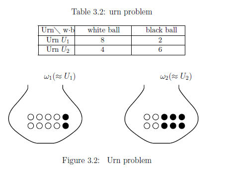
Review 3.16 [= Example 2.34] There are two urns ${U}_1$ and ${U}_2$. The urn ${U}_1$ [resp. ${U}_2$] contains 8 white and 2 black balls [resp. 4 white and 6 black balls] (cf. Figure 3.2).

| $(a):$ | When one ball is picked up from the urn $U_2$, the probability that the ball is white is $0.4$. |
define the state space $\Omega$ by $\Omega = \{ {\omega}_1 , {\omega}_2 \}$ with discrete metric and counting measure $\nu$. That is, we assume the identification;
\begin{align} U_1 \approx \omega_1, \quad U_2 \approx \omega_2, \quad \end{align} Thus, consider the classical basic structure: \begin{align} \mbox{{ $[C_0(\Omega ) \subseteq L^\infty (\Omega, \nu ) \subseteq B(L^2 (\Omega, \nu ))]$} } \end{align}Put "$w$" = "white"$\!\!,\;$ "$b$" = "black"$\!\!\;$, and put $X=\{w,b\}$. And define the observable ${\mathsf O}_{{w}{b}} \big(\equiv (X \equiv \{w,b\}, 2^{\{w,b\}}, F_{{w}{b}}) \big)$ in $L^\infty (\Omega)$ by
\begin{align} [F_{{w}{b}}(\{w\})](\omega_1) = 0.8,& \qquad \qquad [F_{{w}{b}}(\{b\})](\omega_1) = 0.2, \nonumber \\ {}[F_{{w}{b}}(\{w\})](\omega_2) = 0.4,& \qquad \qquad [F_{{w}{b}}(\{b\})](\omega_2) = 0.6. \tag{3.13} \end{align}Thus, we get the measurement $ {\mathsf M}_{L^\infty ({}\Omega{})} ({}{\mathsf O}_{{w}{b}} , S_{[{} \delta_{\omega_2}]})$. Here, Axiom 1 ( $\S$2.7)} says that
| $(b):$ | the probability that a measured value ${w}$ is obtained by ${\mathsf M}_{L^\infty ({}\Omega{})} ({}{\mathsf O}_{{w}{b}} , S_{[{} \delta_{\omega_2}]})$ is given by \begin{align} F_{{w}{b}}(\{b\})(\omega_2) = 0.4 \end{align} |
Thus, the above statement (b) can be rewritten in the terms of quantum language as follows.
| $(c):$ | the probability that a measured value $ \left[\begin{array}{ll} {w} \\ {b} \end{array}\right] $ is obtained by the measurement ${\mathsf M}_{L^\infty (\Omega)} ({\mathsf O}_{{w}{b}} ,$ $ S_{ [{}{\omega_2}]}{})$ is given by $\qquad \qquad \qquad \left[\begin{array}{ll} \int_\Omega [F_{{w}{b}}(\{{w}\})](\omega) \delta_{\omega_2}(d \omega ) = [F_{{w}{b}}(\{{w}\})](\omega_2)= 0.4 \\ \int_\Omega [F_{{w}{b}}(\{{b}\})](\omega) \delta_{\omega_2}(d \omega ) = {[F_{{w}{b}}(\{{b} \})]} (\omega_2)= 0.6 \end{array}\right] $ |
| ${}$ | Pick out one ball from the urn $U_2$, and recognize the color ("white" or "black") of the ball. And the ball is returned to the urn. And again, Pick out one ball from the urn $U_2$, and recognize the color of the ball. Therefore, we have four possibilities such that. \begin{align} ({w},{w})\;\;({w},{b})\;\;({b},{w})\;\;({b},{b})\;\; \end{align} It is a common sense that \begin{align} \mbox{the probability that} \left[\begin{array}{ll} ({w},{w}) \\ ({w},{b}) \\ ({b},{w}) \\ ({b},{b}) \end{array}\right] \mbox{ is given by } \left[\begin{array}{ll} 0.16 \\ 0.24 \\ 0.24 \\ 0.36 \\ \end{array}\right] \end{align} |
| $(a):$ | How do we describe the above fact in term of quantum language? |
Answer It suffices to consider the simultaneous measurement ${\mathsf M}_{L^\infty (\Omega)} ({\mathsf O}^2_{{w}{b}} , S_{ [{}{\delta_{\omega_2}}]}{})$ (= ${\mathsf M}_{L^\infty (\Omega)} ({\mathsf O}_{{w}{b}} \times {\mathsf O}_{{w}{b}} , S_{ [{}{\delta_{\omega_2}}]}{})$ ), where ${\mathsf O}_{{w}{b}}^2 = ( \{ {w}, {b} \}\times \{ {w}, {b} \} , 2^{\{ {w}, {b} \} \times \{ {w}, {b} \} } ,$ $ F_{{w}{b}}^2{}(= F_{{w}{b}} \times F_{{w}{b}} ) )$. Then, we calculate as follows.
\begin{align} & F_{{w}{b}}^2(\{ ({w}, {w}) \}{})(\omega_1{})= 0.64, \qquad F_{{w}{b}}^2(\{ ({w},{b}) \}{})(\omega_1{})= 0.16 \\ & F_{{w}{b}}^2(\{ ({b},{w}) \}{})(\omega_1{})= 0.16, \qquad F_{{w}{b}}^2(\{ ({b},{b}) \}{})(\omega_1{})= 0.4 \end{align} \begin{align} & F_{{w}{b}}^2(\{ ({w}, {w}) \}{})(\omega_2{})= 0.16, \qquad F_{{w}{b}}^2(\{ ({w},{b}) \}{})(\omega_2{})= 0.24 \\ & F_{{w}{b}}^2(\{ ({b},{w}) \}{})(\omega_2{})= 0.24, \qquad F_{{w}{b}}^2(\{ ({b},{b}) \}{})(\omega_2{})= 0.36 \end{align} Thus, we conclude that| $(b):$ | the probability that a measured value
$
\left[\begin{array}{ll}
({w},{w})
\\
({w},{b})
\\
({b},{w})
\\
({b},{b})
\end{array}\right]
$ is obtained by ${\mathsf M}_{L^\infty (\Omega)} ({\mathsf O}_{{w}{b}} \times {\mathsf O}_{{w}{b}} ,
S_{ [{}{\delta_{\omega_2}}]}{})$
is given by $ \left[\begin{array}{llll} {[F_{{w}{b}}(\{{w}\})](\omega_2) \cdot [F_{{w}{b}}(\{{w}\})](\omega_2)=0.16} \\ {[F_{{w}{b}}(\{{w}\})](\omega_2) \cdot [F_{{w}{b}}(\{{b}\})](\omega_2)=0.24} \\ {[F_{{w}{b}}(\{{b}\})](\omega_2) \cdot [F_{{w}{b}}(\{{w}\})](\omega_2)=0.24} \\ {[F_{{w}{b}}(\{{b}\})](\omega_2) \cdot [F_{{w}{b}}(\{{b}\})](\omega_2)=0.36} \end{array}\right] $ |
| ${}$ | Pick out one ball from the urn $U_2$, and recognize the color ("white" or "black") of the ball. And the ball is not returned to the urn. And again, pick out one ball from the urn $U_2$, and recognize the color of the ball. Therefore, we have four possibilities such that. \begin{align} ({w},{w})\;\;({w},{b})\;\;({b},{w})\;\;({b},{b})\;\; \end{align} It is a common sense that \begin{align} \mbox{the probability that} \left[\begin{array}{ll} ({w},{w}) \\ ({w},{b}) \\ ({b},{w}) \\ ({b},{b}) \end{array}\right] \mbox{ is given by } \left[\begin{array}{ll} {12}/{90} \\ {24}/{90} \\ {24}/{90} \\ {30}/{90} \\ \end{array}\right] \end{align} |
Now, we have the following problem:
| $(a):$ | How do we describe the above fact in term of quantum language? |
Now, recall the simultaneous observable (Definition 3.12) as follows. Let ${\mathsf O}_k$ ${{=}}$ $(X_k , $ ${\cal F}_k , $ $F_k{})$ ($k = 1,2,\ldots, n$ ) be observables in $\overline{\mathcal A}$. The simultaneous observable $\widehat{\mathsf O}$ ${{=}}$ $(\times_{k=1}^n X_k ,$ $ \boxtimes_{k=1}^n{\cal F}_k , $ $\widehat{F}{})$ is defined by
\begin{align} {\widehat F}(\Xi_1 \times \Xi_2 \times \cdots \times \Xi_n{}) = F_1 (\Xi_1{}) F_2 (\Xi_2{}) \cdots F_n (\Xi_n{}) \\ (\forall \Xi_k \in {\cal F}_k , \forall k =1,2,\ldots,n ) \end{align} The following definition ("quasi-product observable") is a kind of simultaneous observable:Definition 3.19 [quasi-product{ observable ] Let ${\mathsf O}_k$ ${{=}}$ $(X_k , $ ${\cal F}_k , $ $F_k{})$ ($k = 1,2,\ldots, n$ ) be observables in a $W^*$-algebra $\overline{\mathcal A}$. Assume that an observable ${\mathsf O}_{12...n}$ ${{=}}$ $(\times_{k=1}^n X_k ,$ $ \boxtimes_{k=1}^n{\cal F}_k , $ ${F}_{12...n}{})$ satisfies
\begin{align} & {F}_{12...n}(X_1 \times \cdots \times X_{k-1} \times \Xi_k \times X_{k+1} \times \cdots \times X_n ) = F_k (\Xi_k{}) \tag{3.14} \\ & \quad \qquad \qquad (\forall \Xi_k \in {\cal F}_k , \forall k =1,2,\ldots,n ) \end{align}The observable ${\mathsf O}_{12...n}$ ${{=}}$ $(\times_{k=1}^n X_k ,$ $ \boxtimes_{k=1}^n{\cal F}_k , $ ${F}_{12...n}{})$ is called a quasi-product{ observable of $\{ {\mathsf O}_k \; | \;k=1,2,\ldots,n \}$, and denoted by
\begin{align} {\mathop{\overset{qp}{\times}}_{k=1,2,\ldots,n}}{\mathsf O}_k = (\times_{k=1}^n X_k , \boxtimes_{k=1}^n{\cal F}_k, {\mathop{\overset{qp}{\times}}_{k=1,2,\ldots,n} }F_k{}) \end{align}Of course, a simultaneous observable is a kind of quasi-product observable. Therefore, quasi-product observable is not uniquely determined. Also, in quantum systems, the existence of the quasi-product observable is not always guaranteed.
Answer 3.20 [The answer to Problem 3.18]Define the quasi-product observable $ {\mathsf O}_{{w}{b}} \mathop{\overset{qp}{\times}} {\mathsf O}_{{w}{b}} = ( \{ {w}, {b} \} \times \{ {w}, {b} \} , 2^{\{ {w}, {b} \} \times \{ {w}, {b} \} } ,$ $ F_{12}(= F_{{w}{b}} \mathop{\overset{qp}{\times}} F_{{w}{b}} ))$ of ${\mathsf O}_{{w}{b}} = ( \{ {w}, {b} \}, 2^{\{ {w}, {b} \} } , F{})$ in $L^\infty (\Omega{})$ such that
\begin{align} & F_{12}(\{ ({w}, {w}) \}{})(\omega_1{})= \frac{8 \times 7}{90}, \qquad F_{12}(\{ ({w},{b}) \}{})(\omega_1{})= \frac{8 \times 2}{90} \\ & F_{12}(\{ ({b},{w}) \}{})(\omega_1{})= \frac{2 \times 8}{90}, \qquad F_{12}(\{ ({b},{b}) \}{})(\omega_1{})= \frac{2 \times 1}{90} \\ & F_{12}(\{ ({w}, {w}) \}{})(\omega_2{})= \frac{4 \times 3}{90}, \qquad F_{12}(\{ ({w},{b}) \}{})(\omega_2{})= \frac{4 \times 6}{90} \\ & F_{12}(\{ ({b},{w}) \}{})(\omega_2{})= \frac{6 \times 4}{90}, \qquad F_{12}(\{ ({b},{b}) \}{})(\omega_2{})= \frac{6 \times 5}{90} \end{align}Thus, we have the (quasi-product) measurement ${\mathsf M}_{L^\infty (\Omega)} ({\mathsf O}_{12}, S_{ [{}{\omega}]}{})$ Therefore, in terms of quantum language, we describe as follows.
| $(b):$ | the probability that a measured value $
\left[\begin{array}{ll}
({w},{w})
\\
({w},{b})
\\
({b},{w})
\\
({b},{b})
\end{array}\right]
$ is obtained dy ${\mathsf M}_{L^\infty (\Omega)} ({\mathsf O}_{{w}{b}} \mathop{\overset{qp}{\times}} {\mathsf O}_{{w}{b}} , S_{ [{}{\delta_{\omega_2}}]}{})$
is given by $ \left[\begin{array}{lll} {[F_{12}(\{ ({w}, {w}) \})](\omega_2) =\frac{4 \times 3}{90} } \\ \\ { [F_{12}(\{({w}, {b})\})](\omega_2) =\frac{4 \times 6}{90} } \\ \\ { [ F_{12}(\{ ({b}, {w}) \})](\omega_2) =\frac{4 \times 6}{90} } \\ \\ { [F_{12}(\{({b}, {b}) \}{})](\omega_2) =\frac{6 \times 5}{90} } \end{array}\right] $ |
