3.3.3: Only one state and parallel measurement
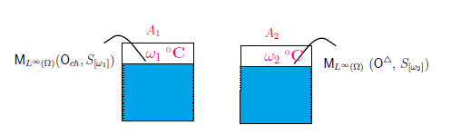
$(a):$ There are two cups $A_1$ and $A_2$ in which water is filled. Assume that the temperature of the water in the cup $A_k$ $(k=1,2)$ is $\omega_k $ °C $(0 {{\; \leqq \;}}\omega_k {{\; \leqq \;}}100)$. Consider two questions "Is the water in the cup $A_1$ cold or hot?" and
"How many degrees(°C) is roughly the water in the cup $A_2$?". This implies that we take two measurements such that
$\quad$ $
\left\{\begin{array}{ll}
\mbox{
$(\sharp_1)$:
${\mathsf M}_{L^\infty ( \Omega )} ( {\mathsf O}_{{{{{c}}}}{{{{h}}}}}
{{=}}
(\{{{{{c}}}},{{{{h}}}}\}
, 2^{\{{{{{c}}}},{{{{h}}}}\}}, F_{{{{{c}}}}{{{{h}}}}} ), S_{[\omega_1]} )$
in Example 2.31}
\\
\\
\mbox{
$(\sharp_2)$
:
${\mathsf M}_{L^\infty ( \Omega )}$
$ ({\mathsf O}^{\triangle}
$
$
{{=}}
({\mathbb N}_{10}^{100} ,$
$
2^{{\mathbb N}_{10}^{100} }, G^{\triangle} ),$
$
S_{[\omega_2]} )
$
in
Example2.32
}
\end{array}\right.
$
This will be answered in what follows.
Definition 3.22 [ Parallel observable] For each $k = 1,2,\ldots,n$, consider a basic structure $[{\mathcal A}_k \subseteq \overline{\mathcal A}_k \subseteq B(H_k)]$, and an observable ${\mathsf O}_k$ $=$ $(X_k , {\cal F}_k , F_k{})$ in $\overline{\mathcal A}_k$. Define the observable $\widetilde{\mathsf O}= ( {\times_{k=1}^n X_k }, \boxtimes_{k=1}^n {\cal F}_k , \widetilde{F}{})$ in $ \bigotimes_{k=1}^n \overline{\mathcal A}_k $ such that
\begin{align} & {\widetilde F}(\Xi_1 \times \Xi_2 \times \cdots \times \Xi_n{}) = F_1 (\Xi_1{}) \otimes F_2 (\Xi_2{}) \otimes \cdots \otimes F_n (\Xi_n{}) \tag{3.15} \\ & \qquad \;\; \forall \Xi_k \in {\cal F}_k \; (k=1,2,\ldots,n ) \nonumber \end{align}Then, the observable $\widetilde{\mathsf O}$ $=$ $(\times_{k=1}^n X_k , \boxtimes_{k=1}^n{\cal F}_k , \widetilde{F}{})$ is called the parallel observable in $ \bigotimes_{k=1}^n \overline{\mathcal A}_k $, and denoted by ${\widetilde F}=\bigotimes_{k=1}^n F_k$, $\widetilde{\mathsf O}$ $=$ $\bigotimes_{k=1}^n {\mathsf O}_k $. the measurement of the parallel observable ${\widetilde{\mathsf O}}=$ $\bigotimes_{k=1}^n {\mathsf O}_k$, that is, the measurement ${\mathsf M}_{ \bigotimes_{k=1}^n \overline{\mathcal A}_k}$ $ (\widetilde{\mathsf O}, $ $S_{ [\bigotimes_{k=1}^n \rho_k] })$ is called a parallel measurement and denoted by ${\mathsf M}_{ \bigotimes_{k=1}^n \overline{\mathcal A}_k} ( \bigotimes_{k=1}^n {\mathsf O}_k,$ $ S_{[ \bigotimes_{k=1}^n \rho_k]})$ or $\bigotimes_{k=1}^n {\mathsf M}_{\overline{\mathcal A}_k} ({\mathsf O}_k,$ $S_{[ \rho_k]})$.
The meaning of the parallel measurement is as follows.
| ${}$ | to take both measurements ${\mathsf M}_{\overline{\mathcal A}_1 }({\mathsf O}_1, S_{[\rho_1]})$ and ${\mathsf M}_{\overline{\mathcal A}_2 }({\mathsf O}_2, S_{[\rho_2]})$ |
| $(b):$ | $ \left\{\begin{array}{ll} \overset{{}}{\underset{ \rho_1 (\in {\frak S}^p({\mathcal A}_1^*) )} {{ \fbox{state}}}} \xrightarrow[]{\qquad \qquad} \overset{{}} { \underset{ {\mathsf O}_1} {{ \fbox{observable}}} } \xrightarrow[{\mathsf M}_{\overline{\mathcal A}_1 }({\mathsf O}_1, S_{[{\rho_1}]})]{\qquad \qquad} \overset{{}} { \underset{ x_1 (\in X_1 )} {{ \fbox{measured value}}} } \\ \\ \overset{{}}{\underset{ \rho_2 (\in {\frak S}^p({\mathcal A}_2^*))} {{ \fbox{state}}}} \xrightarrow[]{\qquad \qquad} \overset{{}} { \underset{ {\mathsf O}_2} {{ \fbox{observable}}} } \xrightarrow[{\mathsf M}_{\overline{\mathcal A}_2}({\mathsf O}_2, S_{[{\rho_2}]})]{\qquad \qquad} \overset{{}} { \underset{ x_2 (\in X_2 )} {{ \fbox{measured value}}} } \end{array}\right. $ |
| $(c):$ | $ \overset{{}}{\underset{ \rho_1 \otimes \rho_2 (\in {\frak S}^p({\mathcal A}_1^*) \otimes {\frak S}^p({\mathcal A}_2^*) ) } {{ \fbox{state}}}} \xrightarrow[]{} { \underset{ {\mathsf O}_1 \otimes {\mathsf O}_2} {{ \fbox{parallel observable}}} } \xrightarrow[ {\mathsf M}_{ \overline{\mathcal A}_1 \otimes \overline{\mathcal A}_2 }({\mathsf O}_1 \otimes {\mathsf O}_2 , S_{[ \rho_1 \otimes \rho_2 ]})] {\qquad \qquad} { \underset{ (x_1,x_2) (\in X_1 \times X_2 )} {{ \fbox{measured value}}} } $ |
 Example 3.23 [The answer to Problem 3.21]
Put $\Omega_1 = \Omega_2 = [0,100]$, and define the state space $\Omega_1 \times \Omega_2$. And consider two observables, that is, the [C-H]-observable ${\mathsf O}_{{{{{c}}}}{{{{h}}}}}= (X {{=}} \{ {{{{c}}}} , {{{{h}}}} \}, 2^X, F_{{{{{c}}}}{{{{h}}}}} )$ in $L^\infty (\Omega_1)$ (in Example 2.31) and triangle-observable ${\mathsf O}^{\triangle}= (Y( {{=}} {\mathbb N}_{10}^{100}) , 2^Y, G^{\triangle} )$ in $L^\infty(\Omega_2)$ (in Example 2.32). Thus, we get the parallel observable ${\mathsf O}_{{{{{c}}}}{{{{h}}}}} \otimes {\mathsf O}^{\triangle}$ $=$ $(\{ {{{{c}}}} , {{{{h}}}} \}\times {\mathbb N}_{10}^{100}, 2^{\{ {{{{c}}}} , {{{{h}}}} \}\times {\mathbb N}_{10}^{100}}, F_{{{{{c}}}}{{{{h}}}}} \otimes G^{\triangle} )$ in $L^\infty (\Omega_1 \times \Omega_2 )$, take the parallel measurement ${\mathsf M}_{L^\infty (\Omega_1 \times \Omega_2 )}({\mathsf O}_{{{{{c}}}}{{{{h}}}}} \otimes {\mathsf O}^{\triangle}, S_{[(\omega_1,\omega_2)]})$. Here, note that
Example 3.23 [The answer to Problem 3.21]
Put $\Omega_1 = \Omega_2 = [0,100]$, and define the state space $\Omega_1 \times \Omega_2$. And consider two observables, that is, the [C-H]-observable ${\mathsf O}_{{{{{c}}}}{{{{h}}}}}= (X {{=}} \{ {{{{c}}}} , {{{{h}}}} \}, 2^X, F_{{{{{c}}}}{{{{h}}}}} )$ in $L^\infty (\Omega_1)$ (in Example 2.31) and triangle-observable ${\mathsf O}^{\triangle}= (Y( {{=}} {\mathbb N}_{10}^{100}) , 2^Y, G^{\triangle} )$ in $L^\infty(\Omega_2)$ (in Example 2.32). Thus, we get the parallel observable ${\mathsf O}_{{{{{c}}}}{{{{h}}}}} \otimes {\mathsf O}^{\triangle}$ $=$ $(\{ {{{{c}}}} , {{{{h}}}} \}\times {\mathbb N}_{10}^{100}, 2^{\{ {{{{c}}}} , {{{{h}}}} \}\times {\mathbb N}_{10}^{100}}, F_{{{{{c}}}}{{{{h}}}}} \otimes G^{\triangle} )$ in $L^\infty (\Omega_1 \times \Omega_2 )$, take the parallel measurement ${\mathsf M}_{L^\infty (\Omega_1 \times \Omega_2 )}({\mathsf O}_{{{{{c}}}}{{{{h}}}}} \otimes {\mathsf O}^{\triangle}, S_{[(\omega_1,\omega_2)]})$. Here, note that
| $(d):$ | When the parallel measurement ${\mathsf M}_{L^\infty (\Omega_1 \times \Omega_2 )}({\mathsf O}_{{{{{c}}}}{{{{h}}}}} \otimes {\mathsf O}^{\triangle}, S_{[(25,55)]})$ is taken, the probability \begin{align} & \mbox{that } \mbox{the measured value } \left[\begin{array}{ll} (\mbox{c}, \mbox{about 50°C}) \\ (\mbox{c}, \mbox{about 60°C}) \\ (\mbox{h}, \mbox{about 50°C}) \\ (\mbox{h}, \mbox{about 60°C}) \end{array}\right] \mbox{is obtained is given by} \left[\begin{array}{ll} 0.375 \\ 0.375 \\ 0.125 \\ 0.125 \end{array}\right] \end{align} |
Remark 3.24 Also, for example, putting $(\omega_1,\omega_2 ) =(55, 55)$, we see:
| $(e):$ | the probability that a measured value $ \left[\begin{array}{ll} (\mbox{c}, \mbox{about 50°C}) \\ (\mbox{c}, \mbox{about 60°C}) \\ (\mbox{h}, \mbox{about 50°C}) \\ (\mbox{h}, \mbox{about 60°C}) \end{array}\right] $ is obtained by parallel measurement ${\mathsf M}_{L^\infty (\Omega_1 \times \Omega_2 )}({\mathsf O}_{{{{{c}}}}{{{{h}}}}} \otimes {\mathsf O}^{\triangle}, S_{[(55,55)]})$ is given by $ \left[\begin{array}{ll} 0.125 \\ 0.125 \\ 0.375 \\ 0.375 \end{array}\right] $ |
The following theorem is clear. But, the assertion is significant.
Theorem 3.25 [Ergodic property] For each $k=1,2, \cdots, n$, consider a measurement ${\mathsf M}_{L^\infty ( \Omega)} ( {\mathsf O}_k(:=(X_k,{\mathcal F}_k, F_k)), S_{[\delta_\omega]})$ with the sample probability space $(X_k,{\mathcal F}_k, P_k^{\omega})$. Then, the sample probability spaces of the simultaneous measurement ${\mathsf M}_{L^\infty ( \Omega)} (\times_{k=1}^n {\mathsf O}_k, S_{[\delta_\omega]})$ and the parallel measurement ${\mathsf M}_{L^\infty ( \Omega^n)}$ $ ( \bigotimes_{k=1}^n {\mathsf O}_k , $ $S_{[ \otimes_{k=1}^n \delta_{\omega}]})$ are the same, that is, these are the same as the product probability space
\begin{align} (\times_{k=1}^n X_k,\boxtimes_{k=1}^n{\mathcal F}_k,\bigotimes_{k=1}^n P_k^{\omega}) \tag{3.17} \end{align} Proof. It is clear, and thus we omit the proof.( Also, see Note 3.5 later.)Example 3.26 [The parallel measurement is always meaningful in both classical and quantum systems] The electron $P_1$ has the (spin) state $\rho_1=|u_1 \rangle \langle u_1|$ $\in$ ${\frak S}^p(B({\mathbb C}^2))$ such that
\begin{align} u_1= \left[\begin{array}{l} \alpha_1 \\ \beta_1 \end{array}\right] \quad (\mbox{where, }\|u_1 \|= (|\alpha_1|^2+ |\beta_1|^2)^{1/2}=1) \end{align}Let ${\mathsf O}_z =(X(=\{ \uparrow, \downarrow \} ),2^X, F^z )$ be the spin observable concerning the $z$-axis such that
\begin{align} F^z( \{ \uparrow \}) = \left[\begin{array}{ll} 1 & 0 \\ 0 & 0 \end{array}\right] , \quad F^z( \{ \downarrow \}) = \left[\begin{array}{ll} 0 & 0 \\ 0 & 1 \end{array}\right] \end{align}Thus, we have the measurement ${\mathsf M_{B({\mathbb C}^2)}}({\mathsf O}_z =(X,2^X, F^z ), S_{[\rho_1]})$. The electron $P_2$ has the (spin) state $\rho_2=|u_2 \rangle \langle u_2|$ $\in$ ${\frak S}^p(B({\mathbb C}^2))$ such that
\begin{align} u= \left[\begin{array}{ll} \alpha_2 \\ \beta_2 \end{array}\right] \quad (\mbox{where, }\|u_2 \|= (|\alpha_2|^2+ |\beta_2|^2)^{1/2}=1) \end{align}Let ${\mathsf O}_x =(X,2^X, F^x )$ be the spin observable concerning the $x$-axis such that
\begin{align} F^x( \{ \uparrow \}) = \left[\begin{array}{ll} 1/2 & 1/2 \\ 1/2 & 1/2 \end{array}\right] , \quad F^x( \{ \downarrow \}) = \left[\begin{array}{ll} 1/2 & -1/2 \\ -1/2 & 1/2 \end{array}\right] \end{align}Thus, we have the measurement ${\mathsf M_{B({\mathbb C}^2)}}({\mathsf O}_x =(X,2^X, F^x ), S_{[\rho_2]})$ Then we have the following problem:
| $(a):$ | Two measurements ${\mathsf M_{B({\mathbb C}^2)}}({\mathsf O}_z =(X,2^X, F^z ), S_{[\rho_1 ]})$ and ${\mathsf M_{B({\mathbb C}^2)}}({\mathsf O}_x =(X,2^X, F^x ), S_{[\rho_2 ]})$ are taken simultaneously? |
| $(b):$ | The probability that a $
\mbox{measured value}
\left[\begin{array}{ll}
(
\uparrow,
\uparrow
)
\\
(
\uparrow,
\downarrow)
\\
(\downarrow,
\uparrow
)
\\
(\downarrow,
\downarrow)
\end{array}\right]
$ is obtained by the parallel measurement ${\mathsf M_{B({\mathbb C}^2) \otimes B({\mathbb C}^2)}}({\mathsf O}_z \otimes {\mathsf O}_z, S_{[\rho \otimes \rho
]})$ is given by
$ \qquad \qquad \left[\begin{array}{ll} \langle u, F^z(\{\uparrow \})u \rangle \langle u, F^x(\{\uparrow \})u \rangle =p_1 p_2 \\ \langle u, F^z(\{\uparrow \})u \rangle \langle u, F^x(\{\downarrow \})u \rangle =p_1(1- p_2) \\ \langle u, F^z(\{\downarrow \})u \rangle \langle u, F^x(\{\uparrow \})u \rangle =(1-p_1) p_2 \\ \langle u, F^z(\{\downarrow \})u \rangle \langle u, F^x(\{\downarrow \})u \rangle =(1-p_1) (1- p_2) \end{array}\right] $ where $ p_1=|\alpha_1|^2, \quad p_2=\frac{1}{2}(|\alpha_1|^2 +\widehat{\alpha}_1 \alpha_2 +\alpha_1\widehat{\alpha}_2 + |\alpha_2|^2) $ |
| $\fbox{Note 3.5}$ |
 Theorem 3.25 is rather deep in the following sense. For example, "To toss a coin 10 times" is a simultaneous measurement. On the other hand, "To toss 10 coins once" is characterized as a parallel measurement. The two have the same sample space. That is,
\begin{align}
\mbox{
"spatial average" = "time average"
}
\end{align}
which is called the ergodic property. This means that the two are not distinguished by the sample space and not the measurements (i.e., a simultaneous measurement and a parallel measurement). However, this is peculiar to classical pure measurements. It does not hold in classical mixed measurements and quantum measurement.
Theorem 3.25 is rather deep in the following sense. For example, "To toss a coin 10 times" is a simultaneous measurement. On the other hand, "To toss 10 coins once" is characterized as a parallel measurement. The two have the same sample space. That is,
\begin{align}
\mbox{
"spatial average" = "time average"
}
\end{align}
which is called the ergodic property. This means that the two are not distinguished by the sample space and not the measurements (i.e., a simultaneous measurement and a parallel measurement). However, this is peculiar to classical pure measurements. It does not hold in classical mixed measurements and quantum measurement.
|
