Consider the basic structure
and measurement ${\mathsf M}_{\overline{\mathcal A}} ({\mathsf O}=(X,{\mathcal F},{ F} ), S_{[\rho]})$, which has the sample probability space $(X,{\mathcal F}, P_\rho )$
Note that the existence of the infinite parallel observable $\widetilde{\mathsf O}$ $
(=\bigotimes_{k=1}^\infty
{\mathsf O}
)
$ $=(X^{\mathbb N} ,$ $ \boxtimes_{k=1}^\infty {\cal F} ,$ ${\widetilde F} ({{=}} \bigotimes_{k=1}^\infty F ) )$ in an infinite tensor $W^*$-algebra $\bigotimes_{k=1}^\infty \overline{\mathcal A}$ is assured by Kolmogorov's extension theorem (Corollary 4.2).
For completeness, let us calculate the sample probability space of the parallel measurement $
{\mathsf M}_{\bigotimes_{k=1}^\infty \overline{\mathcal A}} (\widetilde{\mathsf O}
,
S_{[\bigotimes_{k=1}^\infty \rho]})
$ in both cases (i.e., quantum case and classical case):
Consider the measurement ${\mathsf M}_{\overline{\mathcal A}} ({\mathsf O}=(X,{\mathcal F},{ F} ), S_{[\rho]})$ with the sample probability space $(X,{\mathcal F}, P_\rho )$. Then, by Kolmogorov's extension theorem (Corollary 4.2Corollary), we have the infinite parallel measurement:
The sample probability space $(X^{{\mathbb N}},\boxtimes_{k=1}^\infty{\mathcal F},$ $P_{\bigotimes_{k=1}^\infty \rho})$ is characterized by the infinite probability space $(X^{{\mathbb N}},$ $\boxtimes_{k=1}^\infty {\mathcal F},$ ${\bigotimes_{k=1}^\infty P_\rho})$. Furthermore, we see
4.2.1: The sample space of infinite parallel measurement $\bigotimes_{k=1}^\infty{\mathsf M}_{\overline{\mathcal A}} ({\mathsf O}=(X,{\mathcal F},{ F} ), S_{[\rho]})$
[II]:classical system: Without loss of generality, we assume that the state space $\Omega$ is compact, and $\nu(\Omega)=1$ (cf. Note 2.1). Then, the classical infinite tensor basic structure is defined by
\begin{align}
[ C_0(\times_{k=1}^\infty \Omega )
\subseteq
L^\infty (\times_{k=1}^\infty \Omega,
\otimes_{k=1}^\infty \nu)
\subseteq
B(
L^2 (
\times_{k=1}^\infty \Omega,
\otimes_{k=1}^\infty \nu )
)
]
\tag{4.7}
\end{align}
Therefore, the infinite tensor state space is characterized by
\begin{align}
{\frak S}^p(C_0(\times_{k=1}^\infty \Omega)^*)\Big(
\approx \times_{k=1}^\infty \Omega
\Big)
\tag{4.8}
\end{align}
Put $\rho=\delta_\omega$. the sample probability space $(X^{{\mathbb N}},$ $\boxtimes_{k=1}^\infty{\mathcal F},$ $P_{\bigotimes_{k=1}^\infty \rho})$ of the infinite parallel measurement $
{\mathsf M}_{
L^\infty (\times_{k=1}^\infty \Omega,
\otimes_{k=1}^\infty \nu)
} (\otimes_{k=1}^\infty {\mathsf O}= (X^{{\mathbb N}},$ $\boxtimes_{k=1}^\infty{\mathcal F},$ $\otimes{k=1}^\infty { F} ),$ $ S_{[\bigotimes_{k=1}^\infty \rho]})$ is characterized by
\begin{align}
&
P_{\bigotimes_{k=1}^\infty \rho}
(\Xi_1 \times \Xi_2 \times \cdots \times \Xi_n{}
\times(\times_{k=n+1}^\infty X))
=
\times_{k=1}^n
[ F(\Xi_k )](\omega )
\tag{4.9}
\\
&
\quad
(
\;
\forall
\Xi_k \in {\cal F}={\cal F}_\rho, (\;
k=1,2,\ldots, n),
n=1,2,3 \cdots
)
\end{align}
which is equal to the infinite product probability measure $\bigotimes_{k=1}^n P_\rho$.
[III]: Conclusion: Therefore, we can conclude
$(\sharp):$ in both cases, the sample probability space $(X^{{\mathbb N}},$ $\boxtimes_{k=1}^\infty {\mathcal F},$ $P_{\bigotimes_{k=1}^\infty \rho})$ is defined by the infinite product probability space $(X^{{\mathbb N}},$ $\boxtimes_{k=1}^\infty {\mathcal F},$ ${\bigotimes_{k=1}^\infty P_\rho})$
 Summing up, we have the following theorem ( the law of large numbers ).
Theorem 4.5 [The law of large numbers]
That is,we see, almost surely,
\begin{align}
\underset{\mbox{ (population mean)}}{\fbox{$\int_X f(x) P_\rho ( dx )$}}
=
\underset{\mbox{ (sample mean)}}{\fbox{$
\lim_{n \to \infty }
\frac{f(x_1) +
f(x_2) + \cdots + f({x_n})}{n}
$}}
\tag{4.12}
\end{align}
Remark 4.6 [Frequency probability] In the above, consider the case that
\begin{align}
f(x)=\chi_{{}_{\Xi}}(x)=
\left\{\begin{array}{ll}
1 \;\; & (x \in \Xi)
\\
0 \;\; & (x \notin \Xi)
\end{array}\right.
\quad
(\Xi \in {\mathcal F} )
\end{align}
Then, put
\begin{align}
&
D_{\chi_{{}_{\Xi}}}=\Big\{
(x_1,x_2, \ldots ) \in X^{\mathbb N} \;|\;
\lim_{n \to \infty }
\frac{
\sharp
[
\{
k
\;|\;
x_k \in \Xi,
1\le k \le n \}
}{n}
=
P_\rho ( \Xi )
\Big\}
\tag{4.13}
\\
&
\qquad
\mbox{
(where,
$\sharp[A]$
is the number of the elements of the set $A$)
}
\end{align}
Then, it holds that
\begin{align}
P_{\bigotimes_{k=1}^\infty \rho} (D_{\chi_{{}_{\Xi}}})=1
\tag{4.14}
\end{align}
Therefore, the law of large numbers (Theorem 4.5) says that
$(A):$ for any $f \in L^1( X, P_{\rho})$, put
\begin{align}
&
D_f=\Big\{
(x_1,x_2, \ldots ) \in X^{\mathbb N} \;|\;
\lim_{n \to \infty }
\frac{f(x_1) +
f(x_2) + \cdots + f({x_n})}{n}
=
E(f)
\Big\}
\\
&
\qquad
\mbox{
(
where,
$E(f)
=
\int_X f(x) P_\rho ( dx )$
)
}
\end{align}
Then, it holds that
\begin{align}
P_{\bigotimes_{k=1}^\infty \rho} (D_f)=1
\tag{4.11}
\end{align}
$(\sharp):$ the probability in Axiom 1 ( $\S$2.7) can be regarded as "frequency probability"
4.2.2: Mean,variance,unbiased variance
Consider the measurement ${\mathsf M}_{\overline{\mathcal A}} ({\mathsf O}=({\mathbb R}, {\mathcal B}_{\mathbb R}, F), S_{[{}\rho{}] }{})$. Let $( {\mathbb R}, {\mathcal B}_{\mathbb R}, P_\rho )$ be its sample probability space. That is, consider the case that a measured value space $X={\mathbb R}$.
Here, define:
\begin{align}
&{\mbox{ population mean}}(\mu_{\mathsf O}^{\rho}):E[{\mathsf M}_{\overline{\mathcal A}} ({\mathsf O}=({\mathbb R}, {\mathcal B}_{\mathbb R} F), S_{[{}\rho{}] }{})]
=
\int_{\mathbb R} x P_\rho (dx)(=\mu)
\tag{4.15}
\\
&{\mbox{ population variance}}((\sigma_{\mathsf O}^{\rho})^2):\;\; V[{\mathsf M}_{\overline{\mathcal A}} ({\mathsf O}=({\mathbb R}, {\mathcal B}_{\mathbb R} F), S_{[{}\rho{}] }{})]
=
\int_{\mathbb R} (x- \mu )^2 P_\rho (dx)
\tag{4.16}
\end{align}
Assume that
a measured value $(x_1, x_2, x_3,..., x_n ) (\in {\mathbb R}^n)$ is obtained by the parallel measurement $\otimes_{k=1}^n {\mathsf M}_{\overline{\mathcal A}} ({\mathsf O}, S_{[{}\rho{}] }{})$. Put
\begin{align}
&
{\mbox{ sample distribution}}(\nu_n): \nu_n =\frac{
\delta_{x_1}+\delta_{x_2}+ \cdots +\delta_{x_n}}{n}
\in {\mathcal M}_{+1}(X)
\\
&
{\mbox{ sample mean}}(\overline{\mu}_n):{\overline E}[\otimes_{k=1}^n{\mathsf M}_{\overline{\mathcal A}} ({\mathsf O}, S_{[{}\rho{}] }{})]
=\frac{
{x_1}+{x_2}+ \cdots +{x_n}}{n}
(={\overline{\mu}})
\\
&
\qquad \qquad \qquad \qquad \qquad \qquad \qquad
=\int_{\mathbb R} x \nu_n ( dx )
\\
&
{\mbox{ sample variance}}(s^2_n):{\overline V}[\otimes_{k=1}^n{\mathsf M}_{\overline{\mathcal A}} ({\mathsf O}, S_{[{}\rho{}] }{})]
=\frac{(x_1 - \overline{ \mu})^2+(x_2 - \overline{ \mu})^2+ \cdot +(x_2 - \overline{ \mu})^2}{n}
\\
&
\qquad \qquad \qquad \qquad
=\int_{\mathbb R} (x- {\overline \mu })^2 \nu_n ( dx )
\\
&
{\mbox{ unbiased variance}}(u^2_n):{\overline U}[\otimes_{k=1}^n{\mathsf M}_{\overline{\mathcal A}} ({\mathsf O}, S_{[{}\rho{}] }{})]
=\frac{(x_1 - \overline{ \mu})^2+(x_2 - \overline{ \mu})^2+ \cdot +(x_2 - \overline{ \mu})^2}{n-1}
\\
&
\qquad \qquad \qquad \qquad
\qquad \qquad \qquad
=\frac{n}{n-1 }\int_{\mathbb R} (x- {\overline \mu })^2 \nu_n ( dx )
\end{align}
Under the above preparation, we have:
Theorem 4.7 [Population mean,population variance,sample mean,sample variance]
Assume that a measured value $(x_1, x_2, x_3, \cdots ) (\in {\mathbb R}^{\mathbb N})$ is obtained by the infinite parallel measurement $\bigotimes_{k=1}^\infty {\mathsf M}_{\overline{\mathcal A}} ({\mathsf O}=({\mathbb R}, {\mathcal B}_{\mathbb R}, F), S_{[{}\rho{}] }{})$. Then, the law of large numbers (Theorem 4.5 ) says that
\begin{align}
&
{{}{(4.15)}}=
{\mbox{population mean}}(\mu_{\mathsf O}^{\rho})=\lim_{n \to \infty }
\frac{x_1 + x_2 + \cdots + x_n }{n}
=:\overline{\mu}=\mbox{sample mean}
\\
&
{{}{(4.16)}}=
{\mbox{population variance}}(\sigma_{\mathsf O}^{\rho})=\lim_{n \to \infty }
\frac{(x_1-\mu_{\mathsf O}^{\rho})^2 + (x_2-\mu_{\mathsf O}^{\rho})^2 + \cdots + (x_n-\mu_{\mathsf O}^{\rho})^2 }{n}
\nonumber
\\
&
\qquad \qquad
=
\lim_{n \to \infty }
\frac{(x_1-\overline{\mu})^2 + (x_2-\overline{\mu})^2 + \cdots + (x_n-\overline{\mu})^2 }{n}
=:\mbox{sample variance}
\end{align}
Example 4.8 [Spectrum decomposition]
Consider the quantum basic structure
\begin{align}
[{\mathcal C}(H ) \subseteq B(H ) \subseteq B(H )]
\end{align}
Let $A$ be a self-adjoint operator on $H$, which has the spectrum decomposition (i.e., projective observable) ${\mathsf O}_A=({\mathbb R}, {\mathcal B}_{\mathbb R}, F_A)$ such that
\begin{align}
A= \int_{\mathbb R} \lambda F_A (d \lambda )
\end{align}
That is, under the identification:
\begin{align}
\mbox{
self-adjoint operator:
$A$
}
\underset{\mbox{ identification}}{\longleftrightarrow}
\mbox{
spectrum decomposition:${\mathsf O}_A=({\mathbb R}, {\mathcal B}_{\mathbb R},
F_A)$
}
\end{align}
the self-adjoint operator $A$ is regarded as the projective observable ${\mathsf O}_A=({\mathbb R}, {\mathcal B}_{\mathbb R}, F_A)$. Fix the state $\rho_u = |u \rangle \langle u | \in {\frak S}^p({\mathcal Tr}(H))$. Consider the measurement
$
{\mathsf M}_{B(H)} ({\mathsf O}_A
, S_{[{}|u\rangle \langle u |{}] }{})
$.
Then, we see
\begin{align}
&{\mbox{ population mean}}(\mu_{{\mathsf O}_A}^{\rho_u}):E[{\mathsf M}_{B(H)} ({\mathsf O}_A
, S_{[{}|u\rangle \langle u |{}] }{})]
=
\int_{\mathbb R} \lambda \langle u, F_A(d \lambda ) u \rangle
=\langle u, Au \rangle
\tag{4.17}
\\
&{\mbox{ population variance}}((\sigma_{{\mathsf O}_A}^{\rho_u})^2):\;\;V[{\mathsf M}_{B(H)} ({\mathsf O}_A
, S_{[{}|u\rangle \langle u |{}] }{})]
=
\int_{\mathbb R} (\lambda - \langle u, Au \rangle )^2 \langle u, F_A(d \lambda ) u \rangle
\nonumber
\\
&
\qquad \qquad \qquad \qquad \qquad \qquad \qquad \qquad \qquad
=
\| (A - \langle u, Au \rangle)u \|^2
\tag{4.18}
\end{align}
4.2.3: Robertson uncertainty relation
Now we can introduce Robertson's uncertainty principle
4.2: The law of large numbers in quantum language
This web-site is the html version of "Linguistic Copehagen interpretation of quantum mechanics; Quantum language [Ver. 4]" (by Shiro Ishikawa; [home page] )
PDF download : KSTS/RR-18/002 (Research Report in Dept. Math, Keio Univ. 2018, 464 pages)
Contents:
Preparation 4.4
[I]:quantum system:
The quantum infinite tensor basic structure
is defined by
\begin{align}
[ {\mathcal C}(\otimes_{k=1}^\infty H) \subseteq B(\otimes_{k=1}^\infty H)
\subseteq B(\otimes_{k=1}^\infty H)]
\end{align}
Therefore,infinite tensor state space is characterized by
\begin{align}
{\frak S}^p({\mathcal Tr}(\otimes_{k=1}^\infty H))
\subset {\frak S}^m({\mathcal Tr}(\otimes_{k=1}^\infty H))= \overline{\frak S}^m({\mathcal Tr}(\otimes_{k=1}^\infty H))
\tag{4.5}
\end{align}
Since Definition 2.17 says that ${\mathcal F} = {\mathcal F}_\rho $ $( \forall \rho \in
{\frak S}^p({\mathcal Tr}( H))
)$, the sample probability space $(X^{{\mathbb N}},$ $\boxtimes_{k=1}^\infty{\mathcal F},$ $P_{\bigotimes_{k=1}^\infty \rho})$ of the infinite parallel measurement $
{\mathsf M}_{\bigotimes_{k=1}^\infty B(H)} (\otimes_{k=1}^\infty {\mathsf O}= (X^{{\mathbb N}},$ $\boxtimes_{k=1}^\infty{\mathcal F},$ $\otimes{k=1}^\infty { F} ),$ $ S_{[\bigotimes_{k=1}^\infty \rho]})$ is characterized by
\begin{align}
&
P_{\bigotimes_{k=1}^\infty \rho}
(\Xi_1 \times \Xi_2 \times \cdots \times \Xi_n{}
\times(\times_{k=n+1}^\infty X))
=
\times_{k=1}^n
{}_{{}_{{\mathcal Tr}(H)}} \Big( \rho, F(\Xi_k ) \Big){}_{{}_{B(H)}}
\tag{4.6}
\\
&
\quad
(
\;
\forall
\Xi_k \in {\cal F}={\cal F}_\rho, (\;
k=1,2,\ldots, n),
n=1,2,3 \cdots
)
\end{align}
which is equal to the infinite product probability measure $\bigotimes_{k=1}^n P_\rho$.
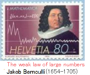
I want to assert that
$$
\left\{\begin{array}{l}
\mbox{The realistic world view started from} \color{red}{\mbox{ Galileo}}
\\
\\
\mbox{The linguistic world view started from } \color{red}{\mbox{ Bernoulli}}
\end{array}\right.
$$
Theorem 4.9 [Robertson's uncertainty principle (parallel measurement)]
Consider the quantum basic structure $[{\mathcal C}(H) \subseteq B(H) \subseteq B(H)]$. Let ${A_1}$ and ${{A_2}}$ be unbounded self-adjoint operators on a Hilbert space $H$, which respectively has the spectrum decomposition:
\begin{align}
{\mathsf O}_{A_1}=({\mathbb R}, {\mathcal B}_{\mathbb R}, F_{A_1})
\;\;
\mbox{ to }
\;\;
{\mathsf O}_{A_1}=({\mathbb R}, {\mathcal B}_{\mathbb R}, F_{A_1})
\end{align}
Thus, we have two measurements ${\mathsf M}_{B(H)}({\mathsf O}_{A_1}, S_{[{\rho_u}]})$ and ${\mathsf M}_{B(H)}({\mathsf O}_{A_2}, S_{[{\rho_u}]})$, where $\rho_u= |u\rangle \langle u |$ $ \in {\frak S}^p({\mathcal C}(H)^*)$. To take two measurements means to take the parallel measurement ${\mathsf M}_{B({\mathbb C}^n)}({\mathsf O}_{A_1}, S_{[{\rho_u}]})$ $\otimes$ ${\mathsf M}_{B({\mathbb C}^n)}({\mathsf O}_{A_2}, S_{[{\rho_u}]})$, namely,
\begin{align}
{\mathsf M}_{B(H)\otimes B(H)}({\mathsf O}_{A_1}\otimes
{\mathsf O}_{A_2}, S_{[{\rho_u} \otimes {\rho_u}]})
\end{align}
Then, the following inequality (i.e., Robertson's uncertainty principle ) holds that
\begin{align}
\sigma_{A_1}^{\rho_u}
\cdot
\sigma_{A_2}^{\rho_u}
{\; \geqq \;}
\frac{1}{2}
|
\langle u , ({A_1}{A_2}-{A_2}{A_1}) u \rangle
|
\qquad
(\forall |u \rangle \langle u |= {\rho_u}, \;\; \| u \|_H=1 )
\end{align}
where $\sigma_{A_1}^{\rho_u}$ and $\sigma_{A_2}^{\rho_u}$ are shown in (4.18), namely,
\begin{align}
\left\{\begin{array}{ll}
\sigma_{A_1}^{\rho_u}
=
\left[
\langle {A_1} u , {A_1} u \rangle
-
|\langle u , {A_1} u \rangle|^2
\right]^{1/2}
=\| (A_1 - \langle u, A_1 u \rangle)u \|
\\
\sigma_{A_2}^{\rho_u}
=
\left[
\langle {A_2} u , {A_2} u \rangle
-
|\langle u , {A_2} u \rangle|^2
\right]^{1/2}
=
\| (A_2 - \langle u, A_2 u \rangle)u \|
\end{array}\right.
\end{align}
Therefore, putting $[A_1, A_2 ] \equiv A_1 A_2 - A_2 A_1$, we rewrite Robertson's uncertainty principle as follows:
\begin{align}
\| A_1 u \|
\cdot
\| A_2 u \|
\ge
\| (A_1 - \langle u, A_1 u \rangle)u \|
\cdot
\| (A_2 - \langle u, A_2 u \rangle)u \|
\ge
| \langle u, [A_1, A_2 ] u \rangle |/2
\tag{4.19}
\end{align}
For example, when $A_1(=Q)$ [resp. $A_2(=P)$ ] is the position observable [resp. momentum observable ] (i.e., $QP-PQ=\hbar {\sqrt{-1}}$), it holds that
\begin{align}
\sigma_Q^{\rho_u}
\cdot
\sigma_P^{\rho_u}
{\; \geqq \;}
\frac{1}{2}
\hbar
\end{align}
Proof.: Robertson's uncertainty principle (4.19) is essentially the same as Schwarz inequality, that is,
\begin{align}
&
|\langle u, [A_1, A_2]u \rangle
|
=
|
\langle u, (A_1 A_2- A_2 A_1)u \rangle
|
\\
=
&
\Big|
\Big\langle u, \Big(
(A_1 -\langle u , A_1 u \rangle )(A_2 -\langle u , A_2 u \rangle )
-
(A_2 -\langle u , A_2 u \rangle )(A_1 -\langle u , A_1 u \rangle )
\Big)
u \Big\rangle
\Big|
\\
\le
&
2
\| (A_1 - \langle u, A_1 u \rangle)u \|
\cdot
\| (A_2 - \langle u, A_2 u \rangle)u \|
\end{align}
