9.8: Averaging information ( Entropy )
As one of applications
(of Bayes theorem),
we now study
the "entropy
of the measurement.
This section is due to the following refs.
Definition 9.19 [Entropy ]
Assume:
Consider
a mixed measurement
${\mathsf M}_{L^\infty(\Omega, \nu )} $
$({\mathsf O} = (X , 2^X , F ), $
$ {\overline S}_{[\ast ]}({w_0}) ) $
with
a countable measured value space $X=\{x_1,x_2,\ldots\}$.
The probability $P(\{ x_n \})$ that
a measured value $x_n$
is obtained by
the mixed measurement ${\mathsf M}_{L^\infty(\Omega)} ({\mathsf O} , {\overline S}_{[\ast ]}({w_0})) $
is given by
Furthermore,
when a measured value $x_n$
is obtained,
the information
$I(\{ x_n \})$
is, from Bayes' theorem 9.11,
is calculated as follows.
Therefore,
the averaging information
$
H
\big( {\mathsf M}_{L^\infty(\Omega)} ({\mathsf O} , {\overline S}_{[\ast ]}({w_0})) \big)
$
of
the mixed measurement
${\mathsf M}_{L^\infty(\Omega)} $
$({\mathsf O}, $
$ {\overline S}_{[\ast ]}({w_0})) $
is naturally defined by
Also,
the following is clear:
Example 9.20 [The offender is man or female?$\;$fast or slow?]
Assume that
Define the state space
$\Omega$
$ = $
$\{ \omega_1 , \omega_2 ,\ldots, \omega_{100} \}$
such that
Assume the counting measure $\nu$ such that
$\nu(\{\omega_k \})=1 (\forall k=1,2, \cdots, 100)$
Define a male-observable
${\mathsf O}_{\rm m}$
$=$
$(X = \{ y_{\rm m} , n_{\rm m} \} , 2^{X} , M )$
in
$L^\infty (\Omega)$
by
For example,
Also,
define
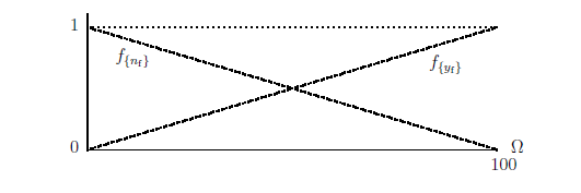
the fast-observable
${\mathsf O}_{\rm f}$
$ = $
$(Y= \{ y_{\rm f} , n_{\rm f} \} , 2^{Y} , F )$
in
$L^\infty(\Omega)$
by

$(\sharp):$
S. Ishikawa,
A Quantum Mechanical Approach to Fuzzy Theory,
Fuzzy Sets and Systems,
Vol. 90, No. 3, 277-306,
1997
$(\sharp):$
S. Ishikawa,
Mathematical Foundations of Measurement Theory,
Keio University Press Inc.
2006.
Let us begin with the following definition.
$(a):$
There are
100 suspected persons
such as
$\{ s_1 , s_2 ,\ldots, s_{100} \}$,
in which
there is one criminal.
$\quad$ Taking a measurement
${\mathsf M}_{L^\infty (\Omega )} ({\mathsf O}_{\rm m} ,
S_{[\omega_{17} ]})
$
---
the sex of the criminal $s_{17}$
---,
we get the measured value $n_{\rm m}$(=female).
According to the principle of equal weight (=Theorem 9.18 ), there is a reason to consider that a mixed state ${w_0}$ $( \in L^1_{+1} (\Omega))$ is equal to the state $w_e$ such that ${w_0} ( \omega_n ) =w_e ( \omega_n ) = 1/100$ $(\forall n)$. Thus, consider two mixed measurement ${\mathsf M}_{L^\infty (\Omega )} ({\mathsf O}_{\rm m} , {\overline S}_{[\ast ]}(w_e)) $ and ${\mathsf M}_{L^\infty (\Omega )} ({\mathsf O}_{\rm f} , {\overline S}_{[\ast ]}(w_e)) $. Then, we see:
\begin{eqnarray*} H \big({\mathsf M}_{L^\infty (\Omega )} ({\mathsf O}_{\rm m} , {\overline S}_{[\ast ]}(w_e))\big) &=& \int_\Omega m_{ y_{\rm m} } (\omega) w_e (\omega ) \nu (d \omega) \cdot \log \int_{\Omega} m_{ y_{\rm m} } (\omega) w_e (\omega ) \nu(d \omega) \\ & & - \int_\Omega m_{\{ n_{\rm m} \} } (\omega) w_e (\omega ) \nu(d \omega) \cdot \log \int_\Omega m_{ n_{\rm m} } (\omega) w_e (\omega ) \nu(d \omega)\\ &=& - \frac{1}{2} \log \frac{1}{2} - \frac{1}{2} \log \frac{1}{2} =\log_2 2 = 1 \; \; \mbox{(bit)} \end{eqnarray*}Also,
\begin{eqnarray*} H \big({\mathsf M}_{L^\infty (\Omega )} ({\mathsf O}_{\rm f} , {\overline S}_{[\ast ]}(w_e)) \big) &=& \int_\Omega f_{ y_{\rm f} } (\omega) \log f_{ y_{\rm f} } (\omega) w_e (\omega ) \nu(d \omega) \\ && \hspace{-4cm}+ \int_\Omega f_{ n_{\rm f} } (\omega) \log f_{ n_{\rm f} } (\omega) w_e (\omega ) \nu(d \omega) - \int_\Omega f_{ y_{\rm f} } (\omega) w_e(\omega ) \nu (d \omega) \cdot \log \int_{\Omega} f_{ y_{\rm f} } (\omega) w_e (\omega ) \nu(d \omega) \\ && \hspace{-4cm} - \int_\Omega f_{ n_{\rm f} } (\omega) w_e (d \omega) \cdot \log \int_\Omega f_{ n_{\rm f} } (\omega) w_e(\omega ) \nu (d \omega) \\ && \hspace{-4cm}{\doteqdot} 2 \int_0^1 \lambda \log_2 \lambda d \lambda +1 = - \frac{1}{ 2 \log_e 2} +1 = 0.278 \cdots \mbox{(bit)} \end{eqnarray*} Therefore, as eyewitness information, "male or female" has more valuable than "fast or slow".