Define the two states space
$\Omega_1$
and
$\Omega_2$
such that
$\Omega_1=\Omega_2={\mathbb R}$ with the Lebesgue measure $\nu$.
Thus we have the classical basic structures:
Define the deterministic causal map
$\phi_{1,2} : \Omega_1 \to \Omega_2 $
such that
Then,
by (10.11),
we get
the deterministic dual
causal operator
${\Phi}^*_{1,2}:{\cal M}_{}(\Omega_1)
\to {\cal M}_{}(\Omega_2) $
such that
where
$\delta_{(\cdot)}$
is the point measure.
Also,
the
deterministic causal operator
$\Phi_{1,2}:L^\infty(\Omega_2)
\to L^\infty (\Omega_1) $
is defined by
Example 10.8 [Dual causal operator, causal operator]
Recall Remark 2.13, that is,
if $\Omega$
$(=\{1,2,...,n \})$
is finite set
( with the discrete metric $d_D$ and the counting measure $\nu$,),
we can consider that
For example,
put
$\Omega_1=\{ \omega_1^1, \omega_1^2, \omega_1^3 \}$
and
$\Omega_2=\{ \omega_2^1 , \omega_2^2\}$.
And define
$\rho_1 (\in {\cal M}_{+1}(\Omega_1))$
such that
Then,
the dual causal operator
${\Phi}^*_{1,2}: {\cal M}_{+1}(\Omega_1) \to {\cal M}_{+1}(\Omega_2)$
is represented by
and,
consider the identification:${\cal M}(\Omega_1) {\; \approx \;} {\mathbb C}^3$,
${\cal M}(\Omega_2) {\; \approx \;} {\mathbb C}^2$,
That is,
Then,
putting
write, by matrix representation,
as follows.
Next, from this dual causal operator
${\Phi}^*_{1,2}: {\cal M}_{}(\Omega_1) \to {\cal M}_{}(\Omega_2)$,
we will construct
a
causal operator
$\Phi_{1,2}: C_0(\Omega_2) \to C_0(\Omega_1)$.
Consider the identification:${C_0}(\Omega_1)
{\; \approx \;}
{\mathbb C}^3$,
${C_0}(\Omega_2) {\; \approx \;} {\mathbb C}^2$,
that is,
Let
$f_2 \in C_0(\Omega_2)$,
$f_1 = \Phi_{1,2} f_2$.
Then,
we see
Therefore,
the relation between
the dual causal operator ${\Phi}^*_{1,2}$
and
causal operator $\Phi_{1,2}$
is represented as the
the transposed matrix.
10.2.2: Simple example---Finite causal operator is represented by
matrix
Example 10.7 [Deterministic causal operator, deterministic dual causal operator, deterministic causal map
]
Example 10.9[Deterministic dual causal operator, deterministic causal map, deterministic causal operator] Consider the case that dual causal operator ${\Phi}^*_{1,2}: {\cal M}(\Omega_1) ({\approx} {\mathbb C}^3) \to {\cal M}(\Omega_2) ({\approx} {\mathbb C}^2) $ has the matrix representation such that
\begin{align} {\Phi}^*_{1,2}(\rho_1 ) = \left[\begin{array}{l} b_1 \\ b_2 \\ \end{array}\right] = \left[\begin{array}{lll} 0 & 1& 1 \\ 1 & 0& 0 \\ \end{array}\right] \left[\begin{array}{l} a_1 \\ a_2 \\ a_3 \\ \end{array}\right] \end{align}In this case, it is the deterministic dual {{causal operator}}. This deterministic causal operator $\Phi_{1,2}: C_0(\Omega_2) \to C_0(\Omega_1)$ is represented by
\begin{align} \left[\begin{array}{l} f_1(\omega_1^1) \\ f_1(\omega_1^2) \\ f_1(\omega_1^3) \\ \end{array}\right] = f_1 = \Phi_{1,2} (f_2 ) = \left[\begin{array}{ll} 0 & 1 \\ 1& 0 \\ 1 & 0 & \\ \end{array}\right] \left[\begin{array}{l} f_2(\omega_2^1) \\ f_2(\omega_2^2) \\ \end{array}\right] \end{align}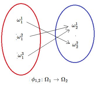
with the deterministic causal map $\phi_{1,2}: \Omega_1 \to \Omega_2$ such that
\begin{align} \phi_{1,2}(\omega_1^1)= \omega_2^2, \quad \phi_{1,2}(\omega_1^2)= \omega_2^1, \quad \phi_{1,2}(\omega_1^3)= \omega_2^1 \quad \end{align} 10.2.3: Sequential causal operator---A chain of causalitiesLet $(T,\le)$ be a finite tree (in Chapter 14, we discuss the infinite case), i.e., a tree like semi-ordered finite set such that "$t_1 \le t_3$ and $t_2 \le t_3$" implies "$t_1 \le t_2$ or $t_2 \le t_1$"
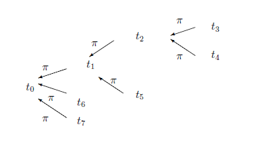
Assume that there exists an element $t_0 \in T$, called the root of $T$, such that $t_0 \le t$ ($\forall t \in T$) holds.
Put $T^2_\le = \{ (t_1,t_2) \in T^2{}: t_1 \le t_2 \}$. An element $t_0 \in T$ is called a root if $t_0 \le t$ ($\forall t \in T$) holds. Since we usually consider the subtree $T_{t_0}$ $(\subseteq T)$ with the root $t_0$, we assume that the tree has a root. In this chapter, assume, for simplicity, that $T$ is finite (though it is sometimes infinite in applications).
For simplicity, assume that $T$ is finite, or a finite subtree of a whole tree. Let $T$ $(= \{ 0, 1, ..., N \})$ be a tree with the root $0$. Define the parent map $\pi{}: T \setminus \{ 0 \} \to T$ such that $\pi (t) = \max \{ s \in T{}: s < t \}$. It is clear that the tree $(T\equiv \{ 0,1,..., N\} , \le)$ can be identified with the pair $(T\equiv \{ 0,1,..., N\} , \pi: T \setminus \{ 0 \} \to T)$. Also, note that, for any $t \in T \setminus \{ 0 \}$, there uniquely exists a natural number $h(t)$ $($called the height of $t$ $)$ such that $\pi^{h(t)} (t) = 0 $. Here, $\pi^2 (t) = \pi (\pi (t))$, $\pi^3 (t) = \pi (\pi^2 (t))$, etc. Also, put $\{ 0,1,..., N \}^2_{{}_{\le}} $ $=$ $\{ (m,n) \; | \; 0 \le m \le n \le N \} $. In Fig.10.2, see the root $t_0$, the parent map: $\pi(t_3)=\pi(t_4)=t_2$, $\pi(t_2)=\pi(t_5)=t_1$, $\pi(t_1)=\pi(t_6)=\pi(t_7)=t_0$
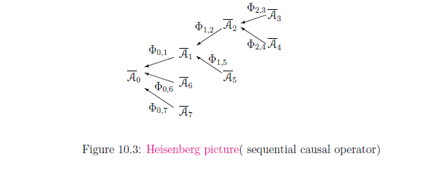
Definition 10.10 [Sequential causal operator; Heisenberg picture of causality]
 The family
$\{ \Phi_{t_1,t_2}{}: $
$ \overline{\mathcal A}_{t_2} \to \overline{\mathcal A}_{t_1} \}_{(t_1,t_2) \in T^2_{\leqq}}$
$\Big($
or,
$\{$
$\overline{\mathcal A}_{t_2} \overset{\Phi_{t_1,t_2}}\to \overline{\mathcal A}_{t_1} \}_{(t_1,t_2) \in T^2_{\leqq}}$
$\Big)$
is called a
sequential causal operator,
if it satisfies that
The family
$\{ \Phi_{t_1,t_2}{}: $
$ \overline{\mathcal A}_{t_2} \to \overline{\mathcal A}_{t_1} \}_{(t_1,t_2) \in T^2_{\leqq}}$
$\Big($
or,
$\{$
$\overline{\mathcal A}_{t_2} \overset{\Phi_{t_1,t_2}}\to \overline{\mathcal A}_{t_1} \}_{(t_1,t_2) \in T^2_{\leqq}}$
$\Big)$
is called a
sequential causal operator,
if it satisfies that
| (i): | For each $t \;(\in T)$, a basic structure $[{\mathcal A}_{t} \subseteq \overline{\mathcal A}_{t} \subseteq B(H_t)] $ is determined. |
| (ii): | For each $(t_1,t_2) \in T^2_{\leqq}$, a {{causal operator}} $\Phi_{t_1,t_2}{}: \overline{\mathcal A}_{t_2} \to \overline{\mathcal A}_{t_1} $ is defined such as $\Phi_{t_1,t_2} \Phi_{t_2,t_3} = \Phi_{t_1,t_3}$ $(\forall (t_1,t_2)$, $\forall (t_2,t_3) \in T^2_{\leqq})$. Here, $\Phi_{t,t} : \overline{\mathcal A}_t \to \overline{\mathcal A}_t$ is the identity operator. |
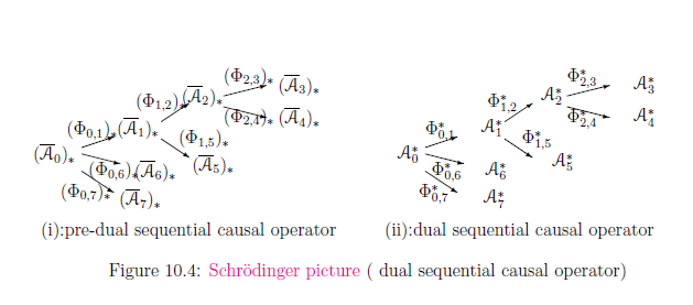
Definition 10.11
(i): [pre-dual sequential causal operator : Schrödinger picture of causality ] The sequence $\{ ({\Phi}_{t_1,t_2})_*{}: $ $ (\overline{\mathcal A}_{t_1})_* \to (\overline{\mathcal A}_{t_1})_* \}_{(t_1,t_2) \in T^2_{\leqq}}$ is called a pre-dual sequential causal operator of $\{ {\Phi_{t_1,t_2}}{}: $ ${ \overline{\mathcal A}_{t_2}} \to {\overline{\mathcal A}{t_1}} \}_{(t_1,t_2) \in T^2_{\leqq}}$
(ii): [Dual sequential causal operator : Schrödinger picture of causality ] A sequence $\{ {\Phi}^*_{t_1,t_2}{}: $ $ {\mathcal A}^\ast_{t_1} \to {\mathcal A}^\ast_{t_1} \}_{(t_1,t_2) \in T^2_{\leqq}}$ is called a dual sequential causal operator of $\{ \Phi_{t_1,t_2}{}: $ ${ \overline{\mathcal A}_{t_2}} \to {\overline{\mathcal A}_{t_1}} \}_{(t_1,t_2) \in T^2_{\leqq}}$.
The Schrödinger picture is intuitive and handy. Consider the Schrödinger picture$\{ {\Phi}^*_{t_1,t_2}{}: $ $ {\mathcal A}^\ast_{t_1} \to {\mathcal A}^\ast_{t_1} \}_{(t_1,t_2) \in T^2_{\leqq}}$. For $C^*$-mixed state $\rho_{t_1} (\in {\frak S}^m({\mathcal A}_{t_1}^*)$ (i.e., a state at time $t_1$),
| $\bullet$ | $C^*$-mixed state $\rho_{t_2} (\in {\frak S}^m({\mathcal A}_{t_2}^*))$ (at time $ t_2 (\ge t_1) $) is defined by \begin{align} \rho_{t_2}=\Phi_{t_1, t_2}^* \rho_{t_1} \end{align} |
However, the linguistic interpretation says "state does not move", and thus, we consider that
| $\bulllet$ | $\left\{\begin{array}{ll} \mbox{ the Heisenberg picture is formal} \\ \\ \mbox{ the Schrödinger picture is makeshift } \end{array}\right. $ |
