10.3:Axiom 2
---Smoke is not located on the place which does not have fire
10.3.1: Axiom 2 (A chain of causal relations)
Now we can propose Axiom 2
(i.e.,
causality),
which is the measurement theoretical representation of
the maxim
(Smoke is not located on the place which does not have fire
):
10.3.2: Sequential causal operator---State equation, etc.
Let $T={\mathbb R}$
be a tree which represents
the time axis.
(Don't mind the infinity of $T$. cf.
Chapter 14.)
For each $t ( \in T)$,
consider the state space
$\Omega_t = {\mathbb R }^n$
($n$-dimensional real space).
And consider
simultaneous ordinary differential equation of the first order.
For each
$t (\in T\mbox{="tree"}))$,
consider the basic structure:
\begin{align}
[{\mathcal A}_t \subseteq \overline{\mathcal A}_t
\subseteq { B(H_t)}]
\end{align}
Then, the
chain of causalities
is represented by
a
sequential causal operator
$ \{ \Phi_{t_1,t_2}{}: $
${\overline{\mathcal A}_{t_2}} \to {\overline{\mathcal A}_{t_1}} \}_{(t_1,t_2) \in T^2_{\leqq}}$.
$\fbox{Note 10.4}$
Axiom 2 (causality) as well as Axiom 1 (measurement)
are kinds of spells.
There are several spells concerning
"motion".
For example,
$(\sharp_1):$
[Aristotle]: final cause
$(\sharp_2):$
[Darwin]: evolution theory(survival of the fittest)
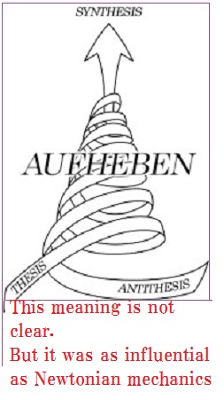
$(\sharp_3):$
[Hegel]: dialectic(Thesis, antithesis, synthesis)
$(\sharp_4):$
law of entropy increase
($\sharp_1$)--($\sharp_3$)
are non-quantitative,
but
($\sharp_4$)
is quantitative.
Nobody disagree that
these
(
($\sharp_1$)--($\sharp_4$)
)
move the world.
In what follows,
we will exercise the chain of causality
in terms of quantum language.
Example 10.13 [State equation]
which is called a state equation. Let $\phi_{t_1,t_2}: \Omega_{t_1} \to \Omega_{t_2}$, $(t_1 {\; \leqq \;} t_2)$ be a deterministic causal map induced by the state equation (10.13). It is clear that $\phi_{t_2,t_3} (\phi_{t_1,t_2} (\omega_{t_1})) = \phi_{t_1,t_3} (\omega_{t_1}) $ $(\omega_{t_1} \in \Omega_{t_1} , t_1 {{\; \leqq \;}}t_2 {{\; \leqq \;}}t_3)$. Therefore, we have the deterministic sequential causal operator $\{ \Phi_{t_1,t_2}{}: $ ${L^\infty (\Omega_{t_2})} \to {L^\infty (\Omega_{t_1})} \}_{(t_1,t_2) \in T^2_{\leqq}}$.
Example 10.14 [Difference equation of the second order]Consider the discrete time $T=\{0, 1 ,2,\ldots \}$ with the parent map $\pi: T\setminus\{0\} \to T$ such that $\pi(t )=t-1 \; (\forall t =1,2,...)$. For each $t ( \in T)$, consider a state space $\Omega_t$ such that $\Omega_t = {\mathbb R }$ ( with the Lebesgue measure). For example, consider the following difference equation, that is, $\phi: \Omega_{t}\times \Omega_{t+1} \to \Omega_{t+2}$ satisfies as follows.
\begin{align} \omega_{t+2} =\phi( \omega_t , \omega_{t+1} ) = \omega_t + \omega_{t+1} +2 \qquad (\forall t \in T ) \end{align}Here, note that the state $\omega_{t+2}$ depends on both $\omega_{t+1}$ and $\omega_{t}$ (i.e., multiple markov property). This must be modified as follows. For each $t ( \in T )$ consider a new state space ${\widetilde \Omega}_t =$ $\Omega_t \times \Omega_{t+1} = {\mathbb R }\times {\mathbb R }$. And define the {{deterministic causal map}} $\widetilde{\phi}_{t,t+1} : {\widetilde \Omega}_t \to {\widetilde \Omega}_{t+1}$ as follows.
\begin{align} & (\omega_{t+1}, \omega_{t+2} ) = \widetilde{\phi}_{t,t+1} (\omega_t, \omega_{t+1} ) = ( \omega_{t+1} , \omega_t + \omega_{t+1} +2 ) \\ & \hspace{5cm} (\forall (\omega_t , \omega_{t+1}) \in {\widetilde \Omega}_t, \forall t \in T ) \end{align}Therefore, by Theorem 10.5, the deterministic causal operator $\widetilde{\Phi}_{t,t+1} : L^\infty({\widetilde \Omega}_{t+1}) \to L^\infty ({\widetilde \Omega}_{t})$ is defined by
\begin{align} & \quad [\widetilde{\Phi}_{t,t+1} {\tilde f}_t]( \omega_t , \omega_{t+1} ) = {\tilde f}_t(\omega_{t+1} , \omega_t + \omega_{t+1} +2 ) \\ & (\forall (\omega_t , \omega_{t+1}) \in {\widetilde \Omega}_t, \forall {\tilde f}_t \in L^\infty ({\widetilde \Omega}_{t+1}) , \forall t \in T\setminus \{0\}) ) \end{align}Thus, we get the deterministic sequential causal operator $\{ {\widetilde{\Phi}}_{t,t+1}{}: $ $L^\infty (\widetilde{\Omega}_{t+1}) \to L^\infty (\widetilde{\Omega}_{t}) \}_{t \in T \setminus \{0\} }$.
| $\fbox{Note 10.5}$ | In order to analyze multiple markov process and time-lag process, such ideas in Example 10.14Example} are needed. |
