In this section, we will analyze a discrete trajectory of a quantum
particle,
which is assumed one of the models of
the Wilson cloud chamber
(
i.e.,
a particle detector used for detecting ionizing radiation).
We will consider a particle $P$ in the one-dimensional real
line ${\mathbb R}$,
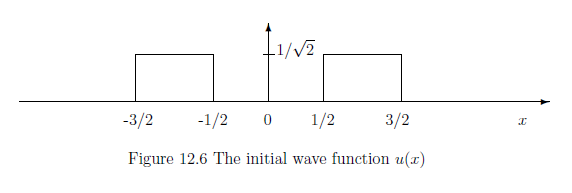
whose initial wave function is $u(x) \in H=L^2({\mathbb R})$.
Since our purpose is to
analyze the discrete trajectory of the particle in the double-slit experiment, we
choose the state $u(x)$
(or precisely,
$| u \rangle \langle u |$
)
as follows:

We treat the following Heisenberg's kinetic equation of the time evolution of the observable $A$, $( -\infty < t < \infty)$ in a Hilbert space $H$ with a Hamiltonian ${\mathcal H}$ such that $ {\mathcal H} = - ( \hbar^2/2m) \partial^2 /\partial x^2 $ (i.e., the potential \( V(x) = 0 \), that is,
\begin{align} - i \hbar \frac{dA_t}{dt} ={\mathcal H} A_t - A_t {\mathcal H}, \quad -\infty < t < \infty, \mbox{ where } A_0=A \tag{12.9} \end{align} The one-parameter unitary group $U_t$ is defined by {$\exp(-itA)$}. An easy calculation shows that \begin{align} A_t = U_t^* AU_t = U^*_txU_t = x +\frac{\hbar t}{im} {\frac{d}{dx}} \tag{12.10} \end{align} Put $t=1/4$, $\hbar/m=1$. And put \begin{align} A=A_0(=x), \qquad B=A_{1/4}(=x+ \frac{1 }{4i} {\frac{d}{dx}}) =U_{1/4}^* A_0U_{1/4}=\Phi_{0, 1/4}A_0 \end{align} Thus, we have the sequential causal observable \begin{align} \underset{\mbox{ initial wave function:$u_0$}}{ \overset{\mbox{ position observable: $A_0$}}{\fbox{$B(H_0)$}}} \xleftarrow[\mbox{ $\quad \Phi_{0,1/4} \quad $}]{} \overset{\mbox{ position observable: $A_0$}}{\fbox{$B(H_{1/4})$}} \end{align} However, $A_0(=A)$ and $\Phi_{0,1/4} A_0(=B)$ do not commute, that is, we see: \begin{align} AB-BA= x (x+ \frac{1 }{4i} {\frac{d}{dx}})-(x+ \frac{1 }{4i} {\frac{d}{dx}})x=i/4 \not=0 \end{align} Therefore, the realized causal observable does not exist. In this sense, \begin{align} \mbox{ the trajectory of a particle is non-sense } \end{align}12.3.2: Approximate measurement of trajectories of a particle
In spite of this fact, we want to consider "trajectories" as follows. That is, we consider the approximate simultaneous measurement of self-adjoint operators $\{A,B \}$ for a particle $P$ with an initial state $u(x)$. Recall Definition 4.13, that is,
Definition 12.12(=Definition 4.13) The quartet $(K, s, \widehat{A}, \widehat{B})$ is called {an approximately simultaneous observable} of $A$ and $B$, if it satisfied that
| $(A_1):$ | $K$ is a Hilbert space. $s \in K$, $\| s \|_K=1$,$\widehat{A}$ and $\widehat{B}$ are commutative self-adjoint operators on a tensor Hilbert space $H \otimes K$ that satisfy the average value coincidence condition, that is, \begin{align} & \langle u \otimes s, {\widehat A}(u \otimes s) \rangle = \langle u , {A} u \rangle, \qquad \langle u \otimes s, {\widehat B}(u \otimes s) \rangle = \langle u , {B} u \rangle \tag{12.11} \\ & \qquad \qquad ( \forall u \in H, \|u\|_H=1) \nonumber \end{align} |
| $(A_2):$ | ${\Delta}_{\widehat{N}_1}^{{\widehat{\rho}_{us}}}$ $(= \| (\widehat{A}-A \otimes I)(u \otimes s) \| )$ and ${ \Delta}_{\widehat{N}_2}^{{\widehat{\rho}_{us}}}$ $(= \| (\widehat{B}-B \otimes I)(u \otimes s) \| )$ are called errors of the approximate simultaneous measurement measurement ${\mathsf{M}}_{B(H\otimes K)} ({\mathsf{O}_{{\widehat A}}}\times{\mathsf{O}_{{\widehat B}}},S_{[{\widehat \rho}_{us}]})$ |
where $\omega_1$ is assumed to be $\omega_1=4,\;16,\;64$ later. It is easy to show that $\| s \|_{L^2({\mathbb R}_y)}=1$ (i.e., $\| s \|_K=1 $ ) and
\begin{align} \langle s, A s \rangle =\langle s, B s \rangle =0 \tag{12.12} \end{align} And further, put \begin{align} & {\widehat A}= A \otimes I + 2 I \otimes A \\ & {\widehat B}= B \otimes I - \frac{1}{2} I \otimes B \end{align} Note that the two commute (i.e., $ {\widehat A}{\widehat B} = {\widehat B}{\widehat A} $ ). Also, we see, by (12.12), \begin{align} & \langle u \otimes s, {\widehat A}(u \otimes s) \rangle = \langle u \otimes s, ( { A}\otimes I +2 I \otimes A) (u \otimes s) \rangle = \langle u , {A} u \rangle \tag{12.13} \\ & \langle u \otimes s, {\widehat A}(u \otimes s) \rangle = \langle u \otimes s, ( { B}\otimes I -2 I \otimes A) (u \otimes s) \rangle = \langle u , {B} u \rangle \tag{12.14} \\ & \qquad ( \forall u \in H, i=1,2) \nonumber \end{align} Thus, we have the approximately simultaneous measurement ${\mathsf{M}}_{B(H\otimes K)} ({\mathsf{O}_{{\widehat A}}}\times{\mathsf{O}_{{\widehat B}}},S_{[{\widehat \rho}_{us}]})$, and the errors are calculated as follows: \begin{align} & \delta_0={\Delta}_{\widehat{N}_1}^{{\widehat{\rho}_{us}}} = \| (\widehat{A}-A \otimes I)(u \otimes s) \| = \| 2(I\otimes A)(u \otimes s) \| = 2\| As\| \tag{12.15} \\ & \delta_{1/4}={ \Delta}_{\widehat{N}_2}^{{\widehat{\rho}_{us}}} = \| (\widehat{B}-B \otimes I)(u \otimes s) \| = (1/2) \| (I\otimes B)(u \otimes s) \| = (1/2)\| Bs\| \tag{12.16} \end{align}By the parallel measurement $\bigotimes_{k=1}^N{\mathsf{M}}_{B(H\otimes K)} ({\mathsf{O}_{{\widehat A}}}\times{\mathsf{O}_{{\widehat B}}},S_{[{\widehat \rho}_{us}]})$, assume that a measured value:
\begin{align} \Big(( x_1, x'_1),(x_2,x'_2), \cdots, (x_N,x'_N)\Big) \end{align} is obtained. This is numerically calculated as follows.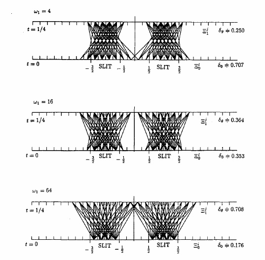
Here, note that $\delta_\theta (=\delta_{1/4})$ and $\delta_0$ are depend on $\omega_1$.
| $\fbox{Note 12.3}$ |
For the further arguments,
see the following refs.
|
