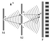
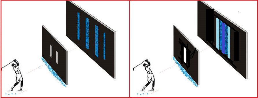
12.2.1. Interference
For each $t \in T=[0, \infty )$, define the quantum basic structure \begin{align*} [{\mathcal C}(H_t) \subseteq B(H_t) \subseteq B(H_t)] , \end{align*} where $H_t=L^2({\mathbb R}^2 )$ $(\forall t \in T)$.
Let $u_0 \in H_0 = L^2({\mathbb R}^2 )$ be an initial wave-function such that ($k_0>0$, small $\sigma > 0$):
\begin{align*} u_0(x,y) \approx \psi_x(x,0) \psi_y (y,0) = \frac{1}{\sqrt{\pi^{1/2}\sigma }} \exp \Big(ik_0 x -\frac{x^2}{2\sigma ^2}\Big) \cdot \frac{1}{\sqrt{\pi^{1/2}\sigma }} \exp \Big(-\frac{y^2}{2\sigma^2}\Big), \end{align*} where the average momentum $(p^0_1,p^0_2)$ is calculated by \begin{align*} (p^0_1,p^0_2)= \Big( \int_{\mathbb R} {\overline \psi}_x(x,0) \cdot \frac{\hbar \partial \psi_x(x,0)}{i \partial x} dx, \int_{\mathbb R} {\overline \psi}_y(y,0) \cdot \frac{\hbar \partial \psi_y(y,0)}{i \partial y} dy \Big) = (\hbar k_0, 0 ). \end{align*} That is, we assume that the initial state of the particle $P$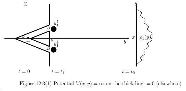
Let $s, t $ be $0 < s < t < \infty $. Thus, we have the causal relation: $ \{ \Phi_{s,t}: B(H_{t}) \to B(H_s) \}_{0 < s < t < \infty } $ where
\begin{align*} & \Phi_{s,t} A =e^{ \frac{{\mathcal H} (t-s) }{i \hbar } } A e^{- \frac{{\mathcal H} (t-s) }{i \hbar } } \qquad (\forall A \in B(H_{t})=B(L^2({\mathbb R}^2 ) ) ) \end{align*} Thus, $(\Phi_{0,t_1})_* (u_0)= u_1^\uparrow + u_1^\downarrow$ in Picture 12.9.Let ${\mathsf O}_2=( {\mathbb R}, {\mathcal B}_{\mathbb R}, F_2)$ be the position observable in $B(L^2({\mathbb R}^2 )$ such that
\begin{align*} [F(\Xi )](x,y) = \chi_{\Xi}( y ) = \begin{cases} 1 \qquad & ( x,y ) \in {\mathbb R} \times \Xi \\ \\ 0 \qquad & ( x,y ) \in {\mathbb R} \times {\mathbb R} \setminus \Xi \end{cases} \end{align*}Hence, we have the measurement ${\mathsf M}_{B(H_0)} (\Phi_{0,t_2} {\mathsf O}_2=( {\mathbb R}, {\mathcal B}_{\mathbb R}, \Phi_{0,t_2} F_2), S_{[|u_0\rangle \langle u_0|]} )$. Axiom 1 ( measurement: $\S$2.7) says that
| $(A):$ | the probability that a measured value $a \in {\mathbb R} $ by ${\mathsf M}_{B(H_0)} (\Phi_{0,t_2} {\mathsf O}, S_{|u_0\rangle \langle u_0|} )$ belongs to $( - \infty , y ]$ is given by $$ \langle u_0 , (\Phi_{0,t_2} F( ( - \infty , y ] )) u_0 \rangle = \int_{- \infty }^y \rho_1 ( y) dy $$ |
| $\fbox{Note 12.3}$ |
Precisely speaking, we say as follows.
Let $\Delta$, $\epsilon$ be small positive real numbers.
For each $k \in {\mathbb Z}=\{k \; | \; k=0, \pm 1, \pm 2, \pm 3, ,,,,\}$, define the rectangle $D_k$ such that
\begin{align*}
&
D_0=\{ (x,y) \in {\mathbb R}^2 \;|\; x < b \},
\\
&
D_k = \{ (x,y) \in {\mathbb R}^2 \;|\; b \le x, (k-1) \Delta < y \le k \Delta \}, \quad k=1,2,3,...
\\
&
D_k = \{ (x,y) \in {\mathbb R}^2 \;|\; b \le x, k \Delta < y \le (k+1) \Delta \}, \quad k=-1,-2,-3,...
\end{align*}
Thus we have the projection observable ${\mathsf O}_2^\Delta
=( {\mathbb Z} , 2^{\mathbb Z}, F_2^\Delta )$ in $L^2({\mathbb R}^2 )$ such that$$
[F(\{k\})](x,y)= 1 \;\; ((x,y) \in D_k), \quad
= 0 \;\; ((x,y) \in {\mathbb R}^2 \setminus D_k)
\qquad ( k \in {\mathbb Z} )
$$
Then it suffices to consider
|
12.2.2. Which-way path experiment
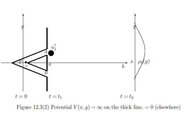
Next, let us explain the above figure. Define the projection observable ${\mathsf O}_1=( \{ \uparrow , \downarrow \}, 2^{ \{ \uparrow , \downarrow \}}, F_1 )$ in $B(L^2( {\mathbb R}^2 ))$ such that
\begin{align*} & [F_1 ( \{ \uparrow \} )](x,y ) = \begin{cases} 1 \qquad & y \ge 0 \\ 0 & y < 0 \end{cases} \\ & [F_1 ( \{ \downarrow \} )](x,y ) = 1- [F_1 ( \{ \uparrow \} )](x,y ) \end{align*}According to Section 11.2 ( Projection postulate ), consider the CONS $\{ e_1, e_2 \}$ $( \in {\mathbb C}^2 )$. Define the predual operator $\Psi_*: Tr(L^2( {\mathbb R}^2 )) \to Tr({\mathbb C}^2 \otimes L^2( {\mathbb R}^2 ))$ such that
$$ \Psi_* ( |u \rangle \langle u | ) = |(e_1 \otimes F_1 (\{ \uparrow \} ) u ) + (e_2 \otimes F_1 (\{ \downarrow \} ) u ) \rangle \langle (e_1 \otimes F_1 (\{ \uparrow \} ) u ) + (e_2 \otimes F_1 (\{ \downarrow \} ) u )| $$Then we have the causal operator $\Psi: B ({\mathbb C}^2 \otimes L^2( {\mathbb R}^2 )) \to L^2( {\mathbb R}^2 )$ such that $\Psi= (\Psi_* )^*$. Define the observable ${\mathsf O}_G =( \{ \uparrow , \downarrow \}, 2^{ \{ \uparrow , \downarrow \}}, G )$ in $B({\mathbb C}^2)$ such that
$$ G( \{ \uparrow \} )= | e_1 \rangle \langle e_1 |, \qquad G( \{ \downarrow \} )= | e_2 \rangle \langle e_2 | $$Hence we have the tensor observable ${\mathsf O}_G \otimes \Phi_{t_1, t_2 } {\mathsf O}_2$ in $B( {\mathbb C}^2 \otimes L^2({\mathbb R}^2 ))$, and hence, the measurement ${\mathsf M}_{B(L^2({\mathbb R}^2 ))} ( \Phi_{0, t_1 } ( \Psi( {\mathsf O}_G \otimes \Phi_{t_1, t_2 } {\mathsf O}_2)), S_{[| u_0 \rangle \langle u_0 |]} )$. Then, Axiom 1 ( measurement: $\S$2.7) says that
| $(B):$ | the probability that a measured value $( \lambda , y ) \in \{\uparrow, \downarrow \} \times {\mathbb R} $ by ${\mathsf M}_{B(L^2({\mathbb R}^2 ))} ( \Phi_{0, t_1 } ( \Psi( {\mathsf O}_G \otimes \Phi_{t_1, t_2 } {\mathsf O}_2)), S_{[| u_0 \rangle \langle u_0 |]} )$ belongs to $\{ \uparrow \} \times ( - \infty , y ]$ is given by $$ \langle u_1^\uparrow , (\Phi_{t_1,t_2} F_2( ( - \infty , y ] )) u_l^\uparrow \rangle = \frac{1}{2} \int_{- \infty }^y \rho_2 ( y) dy $$ |
| $\fbox{Note 12.4}$ | Precisely speaking, in the above case, it suffices to consider the following procedure (1) and (ii): |
| (i): | for time $t_1$, the projection observable ${\mathsf O}_1$ is measured in the sense of Projection Postulate 11.6 |
| (ii): | for each time $t_n = t_2 + n \epsilon (n=0,1,2,...)$, the projection observable ${\mathsf O}_2^\Delta$ is measured in the sense of Projection Postulate 11.6 |
