15.2: Regression analysis in quantum language
Put
$T=\{ 0,1,2, \cdots, i , \cdots, n \}$.
And let $(T, \tau: T \setminus \{0\} \to T )$ be the parallel tree
such that
\begin{align}
\tau(i)=0
\qquad
(\forall i =1,2, \cdots, n)
\tag{15.10}
\end{align}
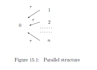
| $\fbox{Note 15.1}$ | In regression analysis, we usually devote ourselves to "classical deterministic causal relation". Thus, Theorem 12.8 is important, which says that it suffices to consider only the parallel structure. |
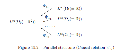
For each $i \in T$, define a locally compact space $\Omega_i$ such that
\begin{align} & \Omega_{0}={\mathbb R}^{2} = \Big\{ \beta =\begin{bmatrix} \beta_0 \\ \beta_1 \\ \end{bmatrix} \;:\; \beta_0, \beta_1 \in {\mathbb R} \Big\} \quad \tag{15.11} \\ & \Omega_{i}={\mathbb R} = \Big\{ \mu_i \;:\; \mu_i \in {\mathbb R} \Big\} \quad(i=1,2, \cdots, n ) \tag{15.12} \end{align} where the Lebesgue measures $m_i$ are assumed.Assume that \begin{align} a_i \in {\mathbb R} \qquad (i=1,2, \cdots, n ), \tag{15.13} \end{align}
which are called explanatory variables in the conventional statistics. Consider the deterministic causal map $\psi_{a_i}: \Omega_0(={\mathbb R}^2) \to \Omega_{i} (={\mathbb R})$ such that
\begin{align} \Omega_0={\mathbb R}^2 \ni \beta =(\beta_0, \beta_1 ) \mapsto \psi_{a_i} ( \beta_0, \beta_1) = \beta_0 + \beta_1 a_i= \mu_i \in \Omega_i ={\mathbb R} \tag{15.14} \end{align}which is equivalent to the deterministic causal operator $\Psi_{a_i}: L^\infty(\Omega_{i}) \to L^\infty(\Omega_0)$ such that
\begin{align} [{\Psi_{a_i}}(f_i)](\omega_0) = f_i( \psi_{a_i} (\omega_0)) \quad (\forall f_i \in L^\infty(\Omega_{i}), \;\; \forall \omega_0 \in \Omega_0, \forall i \in 1,2, \cdots, n) \tag{15.15} \end{align}Thus, under the identification: $a_i \Leftrightarrow \Psi_{a_i}$, the term "explanatory variable" means a kind of causal relation $\Psi_{a_i}$.
For each $i=1,2, \cdots, n$, define the normal observable ${\mathsf O}_{i} {{\equiv}} ({\mathbb R}, {\cal B}_{{\mathbb R}}, G_{\sigma_{}})$ in $L^\infty (\Omega_{i}(\equiv {\mathbb R}))$ such that
\begin{align} & [G_{\sigma_{}}(\Xi)] (\mu ) = \frac{1}{(\sqrt{2 \pi \sigma_{}^2})} \underset{\Xi}{\int} \exp \Big[{- \frac{ (x -\mu )^2 }{2 \sigma_{}^2}} \Big] dx \qquad (\forall \Xi \in {\cal B}_{{\mathbb R}}, \forall \mu \in \Omega_{i} (\equiv {\mathbb R} )) \tag{15.16} \end{align} where $\sigma $ is a positive constant.Thus, we have the observable ${\mathsf O}_{0}^{a_i} {{\equiv}} ({\mathbb R}, {\cal B}_{{\mathbb R}}, \Psi_{a_i}G_{\sigma_{}})$ in $L^\infty (\Omega_{0}(\equiv {\mathbb R}^2))$ such that
\begin{align} & [\Psi_{a_i}(G_{\sigma_{}}(\Xi))] (\beta ) = [(G_{\sigma_{}}(\Xi))] (\psi_{a_i}(\beta )) = \frac{1}{(\sqrt{2 \pi \sigma_{}^2})} \underset{\Xi}{\int} \exp \Big[{- \frac{ (x - (\beta_0 + a_{i{}} \beta_1 ))^2}{2 \sigma_{}^2}} \Big] dx \tag{15.17} \\ & \qquad (\forall \Xi \in {\cal B}_{{\mathbb R}}, \forall \beta =(\beta_0, \beta_1 )\in \Omega_{0} (\equiv {\mathbb R}^{2} ) \nonumber \end{align}Hence, we have the simultaneous observable $\times_{i=1}^n{\mathsf O}_{0}^{a_i} {{\equiv}} ({\mathbb R}^n, {\cal B}_{{\mathbb R}^n}, \times_{i=1}^n \Psi_{a_i}G_{\sigma_{}})$ in $L^\infty (\Omega_{0}(\equiv {\mathbb R}^2))$ such that
\begin{align} & [(\times_{i=1}^n \Psi_{a_i}G_{\sigma_{}}) (\times_{i=1}^n \Xi_i)](\beta) = \times_{i=1}^n \Big( [\Psi_{a_i}G_{\sigma_{}}) (\Xi_i)](\beta)\Big) \nonumber \\ = & \frac{1}{(\sqrt{2 \pi \sigma_{}^2})^n} \underset{\times_{i=1}^n \Xi_i}{\int \cdots \int} \exp \Big[{- \frac{ \sum_{i=1}^n (x_i - (\beta_0 + a_{i{}} \beta_1 ))^2}{2 \sigma_{}^2}} \Big] dx_1 \cdots dx_n \nonumber \\ = & \underset{\times_{i=1}^n \Xi_i}{\int \cdots \int} { p_{(\beta_0, \beta_1, \sigma )} (x_1, x_2, \cdots, x_n ) } dx_1 \cdots dx_n \tag{15.18} \\ & \qquad \qquad \qquad (\forall \times_{i=1}^n \Xi_i \in {\cal B}_{{\mathbb R}^n}, \forall \beta =(\beta_0, \beta_1 ) \in \Omega_{0} (\equiv {\mathbb R}^{2} ) ) \nonumber \end{align}Assuming that $\sigma$ is variable, we have the observable ${\mathsf O}= \Big({\mathbb R}^n(=X) , {\mathcal B}_{{\mathbb R}^n}(={\mathcal F}), F \Big)$ in $L^\infty ( \Omega_0 \times {\mathbb R}_+ )$ such that
\begin{align} [F(\times_{i=1}^n \Xi_i )](\beta, \sigma_) = [(\times_{i=1}^n \Psi_{a_i}G_{\sigma_{}}) (\times_{i=1}^n \Xi_i)](\beta) \quad (\forall \Xi_i \in {\cal B}_{{\mathbb R}}, \forall (\beta , \sigma_{} ) \in {\mathbb R}^2(\equiv \Omega_0) \times {\mathbb R}_+ ) \tag{15.19} \end{align}Assume that a measured value $x=\begin{bmatrix} x_1 \\ x_2 \\ \vdots \\ x_n \end{bmatrix} \in X={\mathbb R}^n $ is obtained by the measurement ${\mathsf M}_{L^\infty(\Omega_{0} \times {\mathbb R}_+)}( {\mathsf O} \equiv (X, {\cal F}, F) , S_{[(\beta_0,\beta_1, \sigma)]} {} )$. (The measured value is also called a response variable .) And assume that we do not know the state $ (\beta_0, \beta_1, \sigma_{}^2 )$.
Then,| $\bullet$ | from the measured value $ x=( x_1, x_2, \ldots, x_n ) \in {\mathbb R}^{n}$, infer the $\beta_0, \beta_1, \sigma_{}$! |
That is, represent the $(\beta_0, \beta_1, \sigma_)$ by $(\hat{\beta}_0(x), \hat{\beta}_1(x), \hat{\sigma}_{}(x))$ (i.e., the functions of $x$).
Answer Taking partial derivatives with respect to $\beta_0$, $\beta_1 $, $\sigma_{}^2$, and equating the results to zero, gives the $\log$-likelihood equations. That is, putting
\begin{align} L(\beta_0, \beta_1, \sigma^2, x_1, x_2, \cdots, x_n)=\log \Big( p_{(\beta_0, \beta_1, \sigma )} (x_1, x_2, \cdots, x_n ) \Big), \end{align}(where "$\log$" is not essential), we see that
\begin{align} & \frac{\partial L}{\partial \beta_0}=0 \quad \Longrightarrow \quad {\sum_{i=1}^n {(x_i - (\beta_0 + {{}} a_{i{}} \beta_1 ))} } =0 \tag{15.20} \\ & \frac{\partial L}{\partial \beta_1}=0 \quad \Longrightarrow \quad {\sum_{i=1}^n {a_{i{}}(x_i - (\beta_0 + {{}} a_{i{}} \beta_1 ))} } =0 \tag{15.21} \\ & \frac{\partial L}{\partial \sigma^2}=0 \quad \Longrightarrow -\frac{n}{2\sigma_{}^2} + \frac{1}{2\sigma_{}^4} {\sum_{i=1}^n (x_i - \beta_0 - \beta_1 a_i)^2 } =0 \tag{15.22} \end{align}Therefore, using the notations (15.7)-(15.9), we obtain that
\begin{align} & \hat{\beta}_0(x)=\overline{x} -\hat{\beta}_1(x) \overline{a}=\overline{x} -\frac{s_{ax}}{s_{aa}} \overline{a}, \quad \hat{\beta}_1(x)=\frac{s_{ax}}{s_{aa}} \tag{15.23} \end{align} and \begin{align} & (\hat{\sigma_{}}(x))^2= \frac{\sum_{i=1}^n \Big( x_i - ( \hat{\beta}_0 (x)+ a_{i{}} \hat{\beta}_1 (x) ) \Big)^2}{n} \nonumber \\ = & \frac{\sum_{i=1}^n \Big( x_i - ( \overline{x} -\frac{s_{ax}}{s_{aa}} \overline{a}) - a_i \frac{s_{ax}}{s_{aa}} \Big)^2}{n} = \frac{\sum_{i=1}^n \Big(( x_i - \overline{x}) +( \overline{a} - a_i) \frac{s_{ax}}{s_{aa}} \Big)^2}{n} \nonumber \\ = & s_{xx} - 2 s_{ax}\frac{s_{ax}}{s_{aa}} + s_{aa}(\frac{s_{ax}}{s_{aa}})^2 = s_{xx} - \frac{s_{ax}^2}{s_{aa}} \tag{15.24} \end{align}Note that the above (15.23) and (15.24) are the same as (15.6). Therefore, Problem 15.3 (i.e., regression analysis in quantum language) is a quantum linguistic story of the least squares method (Problem 15.1).
Remark 15.4 Again,note that
| $(A):$ | the least squares method (15.6) and the regression analysis (15.23) and (15.24) are the same. |
Therefore, a small mathematical technique (the least squares method) can be understood in a grand story (regression analysis in quantum language). The readers may think that
| $(B):$ | Why do we choose "complicated (Problem 15.3)" rather than "simple (Problem 15.1)"? |
Of course, such a reason is unnecessary for quantum language! That is because
| $(C):$ |
the spirit of quantum language says that
|
However, this may not be a kind answer. The reason is that the grand story has a merit such that statistical methods (i.e., the confidence interval method and the statistical hypothesis testing ) can be applicable. This will be mentioned in the following section.
