2.8.1: Linguistic world-view ---Wonder of man's linguistic competence
The applied scope of physics physics (realistic world-description method) is rather clear. But the applied scope of mea urement theory is ambiguous.
What we can do in measurement theory (= quantum language) is
(a): $ \left\{\begin{array}{ll}
\mbox{(a$_1$): Use the language defined by Axiom 1 ( $\S$2.7)
}
\\
\\
\mbox{(a$_2$):
Trust in man's linguistic competence
}
\end{array}\right.
$

| (b): | $\qquad \qquad$ Is it science? |
2.8.2 Elementary examples---urn problem, etc.
Since measurement theory is a language, we can not master it without exercise. Thus, we present simple examples in what follows.
Example 2.32 [ The measurement of the approximate temperature of water in a cup (continued from Example 2.22: triangle observable)] Consider the classical basic structure: \begin{align*} \mbox{ $[C_0(\Omega ) \subseteq L^\infty (\Omega, \nu ) \subseteq B(L^2 (\Omega, \nu ))]$ } \end{align*}
where $\Omega =$"the closed interval $[0, 100]$" with the Lebesgue measure $\nu$.
 Let testees drink water with various temperature $\omega $ °C $(0 {{\; \leqq \;}}\omega {{\; \leqq \;}}100)$.
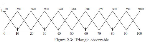
And you ask them "How many degrees(°C) is roughly this water?" Gather the data, ( for example, $h_{n}(\omega)$ persons say $n $ °C ${(}n=0,10,20,\ldots,90,100)$. and normalize them, that is, get the polygonal lines. For example, define the state space $\Omega$ by the closed interval $[0,100]$ $( \subseteq {\mathbb R})$ with the Lebesgue measure. For each $n \in {\mathbb N}_{10}^{100} = \{0,10,20,\ldots,100\}$, define the (triangle) continuous function $g_{n}:\Omega \to [0,1]$ by

| (a): | You choose one person from the testees, and you ask him/her "How many degrees(°C) is roughly this water?". Then the probability that he/she says $ \left[\begin{array}{ll} {} \mbox{"about 40°C"} \\ {} \mbox{"about 50°C"} \end{array}\right] $ is given by $ \left[\begin{array}{ll} {}g_{\text 40}(47)=0.25 \\ {} f_{\text 50}(47)=0.75 \end{array}\right] $ |
This is described in terms of Axiom 1 ( $\S$2.7) in what follows. Putting $Y={\mathbb N}_{10}^{100}$, define the triangle observable ${\mathsf O}^{\triangle}= (Y , 2^Y, G^{\triangle} )$ in $L^\infty (\Omega )$ such that
\begin{align*} & [G^{\triangle}(\emptyset )](\omega ) = 0, \qquad [G^{\triangle}(Y )](\omega ) = 1 \\ & [G^{\triangle} (\Gamma )](\omega ) = \sum\limits_{n \in \Gamma } g_n (\omega ) \quad \qquad (\forall \Gamma \in 2^{{\mathbb N}_{10}^{100} }, \forall \omega \in \Omega =[0, 100]) \end{align*}Then, we have the triangle observable ${\mathsf O}^{\triangle}= (Y (= {{\mathbb N}_{10}^{100} } ), 2^Y, G^{\triangle} )$ in $L^\infty ([0,100])$. And we get a measurement ${\mathsf M}_{L^\infty ( \Omega )} ( {\mathsf O}^{\triangle}, S_{ [\delta_\omega]} )$. For example, putting $\omega$=47°C, we see, by Axiom 1 ( $\S$2.7), that
| $(b):$ | the probability that a measured value obtained by the measurement $
{\mathsf M}_{L^\infty ( \Omega )} ( {\mathsf O}^{\triangle},$ $S_{[ \omega(=47)]} )$
is $ \left[\begin{array}{ll} {\mbox{about 40°C}} \\ \mbox{about 50°C} \end{array}\right] $ is given by $ \left[\begin{array}{ll} {[G^{\triangle}( \{ 40 \})](47)=0.3} \\ {[G^{\triangle}( \{ 50 \})](47)=0.7} \end{array}\right] $ |
Therefore, we see:
\begin{align} \underset{\mbox{ (ordinary language)}}{\fbox{statement (a)}} \xrightarrow[{\mbox{ translation}}]{} \underset{\mbox{ (quantum language)}}{\fbox{statement (b)}} \tag{2.69} \end{align}Example 2.33 [Exact measurement] Consider the classical basic structure: \begin{align*} \mbox{{ $[C_0(\Omega ) \subseteq L^\infty (\Omega, \nu ) \subseteq B(L^2 (\Omega, \nu ))]$} } \end{align*}

Let ${\mathcal B}_\Omega$ be the Borel field. Then, define the exact observable ${\mathsf O}^{{ (exa)}} = (X(=\Omega) , {\mathcal F}(={\mathcal B}_\Omega), F^{\rm (exa)}{})$ in $ L^\infty (\Omega, \nu ) $ such that
\begin{align*} [F^{\rm (exa)}(\Xi)](\omega) = \chi_{{}_\Xi} (\omega) = \left\{\begin{array}{ll} 1 \quad & ( \omega \in \Xi )\\ \\ 0 & ( \omega \notin \Xi ) \end{array}\right. \qquad (\forall \Xi \in {\mathcal B}_\Omega{}) \end{align*}Let $\delta_{\omega_0 } \approx \omega_0 (\in \Omega )$. Consider the exact measurement ${\mathsf M}_{L^\infty ( \Omega, \nu )} ( {\mathsf O}^{{ (exa)}}, S_{[\delta_{\omega_0} ]})$. Here, Axiom 1 ($\S$2.7) says:
| (a): | Let $D (\subseteq \Omega)$ be arbitrary open set such that $\omega_0 \in D$. Then, the probability that a measured value obtained by the exact measurement ${\mathsf M}_{L^\infty ( \Omega, \nu )} ({\mathsf O}^{ (exa)}, S_{[\delta_{\omega_0 }]})$ belongs to $D$ is given by \begin{align*} {{}_{C_0(\Omega)^*}} \Big( \delta_{{\omega_0}}, \chi_{{}_D} \Big){{}_{L^\infty(\Omega, \nu )}} = 1 \end{align*} |
| $(b):$ | a measured value $\omega_0$ is, with the probability $1$, obtained by the exact measurement ${\mathsf M}_{L^\infty ( \Omega, \nu )}$ $ ( {\mathsf O}^{ (exa)},$ $ S_{[\delta_{\omega_0 }]})$. |
Then, when $\Xi \in {\mathcal F}_{\omega_0} $, $F(\Xi)$ is continuous at $\omega_0$. And, ${\mathcal F}$ is the smallest $\sigma$-field that contains ${\mathcal F}_{\omega_0}$.{\;\;} Therefore, we have the probability space $(X, {\mathcal F}, P_{\delta_{\omega_0}})$ such that
\begin{align*} P_{\delta_{\omega_0}}( \Xi ) = [F(\Xi )](\omega_0 ) \qquad (\forall \Xi \in {\mathcal F}_{\omega_0}) \end{align*} that is,| $(c):$ | the exact measurement ${\mathsf M}_{L^\infty ( \Omega, \nu )} ( {\mathsf O}^{ (exa)}, S_{[\delta_{\omega_0 }]})$ has the sample space $(X, {\mathcal F}, P_{\delta_{\omega_0}})$ $ (= (\Omega,$ $ {\mathcal B_{\Omega}} ,$ $ P_{\delta_{\omega_0}} )) $ |

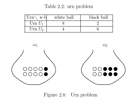
| (a): | When one ball is picked up from the urn $U_2$, the probability that the ball is white is $0.4$. |
define the state space $\Omega$ by $\Omega = \{ {\omega}_1 , {\omega}_2 \}$ with the discrete metric and the {counting measure} $\nu$ (i.e., $\nu(\{\omega_1\})=\nu(\{\omega_2\})=1$). That is, we assume the identification;
\begin{align*} U_1 \approx \omega_1, \quad U_2 \approx \omega_2, \quad \end{align*} Thus, consider the classical basic structure: \begin{align*} \mbox{ $[C_0(\Omega ) \subseteq L^\infty (\Omega, \nu ) \subseteq B(L^2 (\Omega, \nu ))]$ } \end{align*}Put "$w$" = "white"$\!\!,\;$ "$b$" = "black"$\!\!\;$, and put $X=\{w,b\}$. And define the observable ${\mathsf O} \big(\equiv (X \equiv \{w,b\}, 2^{\{w,b\}}, F) \big)$ in $L^\infty (\Omega)$ by
\begin{align*} [F(\{w\})](\omega_1) = 0.8,& \qquad \qquad [F(\{b\})](\omega_1) = 0.2, \\ {}[F(\{w\})](\omega_2) = 0.4,& \qquad \qquad [F(\{b\})](\omega_2) = 0.6. \end{align*}Thus, we get the measurement $ {\mathsf M}_{L^\infty ({}\Omega{})} ({}{\mathsf O} , S_{[{} \delta_{\omega_2}]})$. Here, Axiom 1 ( $\S$2.7) says that
| (b): | the probability that a measured value ${w}$ is obtained by ${\mathsf M}_{L^\infty ({}\Omega{})} ({}{\mathsf O} , S_{[{} \delta_{\omega_2}]})$ is given by \begin{align*} F(\{b\})(\omega_2) = 0.4 \end{align*} |
| $\fbox{Note 2.5}$ | [$L^\infty (\Omega, \nu )$, or in short, $L^\infty (\Omega)$] In the above example, the counting measure $\nu$ (i.e., $\nu(\{\omega_1\})=\nu(\{\omega_2\})=1$) is not absolutely indispensable. For example,even if we assume that $\nu(\{\omega_1\})=2$ and $\nu(\{\omega_2\})=1/3$, we can assert the same conclusion. Thus, in this note, \begin{align*} \mbox{ $L^\infty (\Omega, \nu )$ is often abbreviated to $L^\infty (\Omega)$. } \end{align*} |
| $\fbox{Note 2.6}$ | The statement (a) in Example 2.34 is not necessarily guaranteed, that is,
It is a matter of course that "probability" can not be derived from mathematics itself. For example, the following $(\sharp_1)$ and $(\sharp_2)$ are not guaranteed.
The common sense --- "probability" can not be derived from mathematics itself --- is well known as Bertrand's paradox (cf. $\S$9.12). Thus, it is usual to add the term "at random" to the above $(\sharp_1)$ and $(\sharp_2)$. In this note, this term "at random" is usually omitted. |
 Example 2.35 [Blood type system]
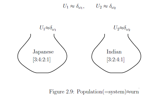
The ABO blood group system is the most important blood type system (or blood group system) in human blood transfusion. Let ${U}_1$ be the whole Japanese's set and let ${U}_2$ be the whole Indian's set. Also, assume that the distribution of the ABO blood group system [O:A:B:AB] concerning Japanese and Indians is determined in Table 2.3.

| (a): | Choose one person from the the whole Indian's set $U_2$ at random. Then the probability that the person's blood type is $ \left[\begin{array}{ll} O \\ A \\ B \\ AB \end{array}\right] $ is given by $ \left[\begin{array}{ll} 0.3 \\ 0.2 \\ 0.4 \\ 0.1 \end{array}\right] $ |
In what follows, we shall translate the statement (a) described in ordinary language to quantum language. Put $\Omega = \{ {\omega}_1 , {\omega}_2 \}$ and consider the discrete metric $(\Omega, d_D)$. We get consider the classical basic structure:
\begin{align*} \mbox{{ $[C_0(\Omega ) \subseteq L^\infty (\Omega, \nu ) \subseteq B(L^2 (\Omega, \nu ))]$} } \end{align*} Therefore, the pure state space is defined by \begin{align*} {\frak S}^p (C_0(\Omega)^*)= \{ \delta_{\omega_1} , \delta_{\omega_2} \} \end{align*} Here, consider \begin{align*} & \delta_{\omega_1} \quad \cdots \quad \mbox{"the state of the whole Japanese's set $U_1$(i.e., population)"} \qquad \\ & \delta_{\omega_2} \quad \cdots \quad \mbox{"the state of the whole India's set $U_1$(i.e., population)"}, \end{align*} Note that "population" = "system" (cf. Table 2.1). That is, we consider the following identification: (Therefore, image Figure 2.9):
Define the blood type observable ${\mathsf O}_{\mbox{ BT}} = ( \{ O, A,B,AB \}, 2^{\{ O, A,B,AB \} } , F_{{{\mbox{ BT}}}}{})$ in $L^\infty (\Omega, \nu )$ such that
\begin{align} & [F_{\mbox{ BT}}(\{ O \}{})](\omega_1{})= 0.3, & \quad & [ F_{\mbox{ BT}}(\{ A \}{})](\omega_1{})= 0.4 \nonumber \\ & [F_{\mbox{ BT}}(\{ B \}{})](\omega_1{})= 0.2, & \quad & [ F_{\mbox{ BT}}(\{ AB \}{})](\omega_1{})= 0.1 \tag{2.71} \end{align} \begin{align} & [F_{\mbox{ BT}}(\{ O \}{})](\omega_2{})= 0.3, & \quad & [F_{\mbox{ BT}}(\{ A \}{})] (\omega_2{})= 0.2 \nonumber \\ & [F_{\mbox{ BT}}(\{ B \}{})](\omega_2{})= 0.4, & \quad & [F_{\mbox{ BT}}(\{ AB \}{})] (\omega_2{})= 0.1 \tag{2.72} \end{align}Thus we get the measurement ${\mathsf M}_{{L^\infty (\Omega, \nu )}} ({\mathsf O}_{{{\mbox{ BT}}}} , S_{ [{}{\delta_{\omega_2}}]}{})$. Hence, the above (a) is translated to the following statement (in terms of quantum language):
| (b): | The probability that a measured value $
\left[\begin{array}{ll}
O
\\
A
\\
B
\\
AB
\end{array}\right]
$ is obtained by the measurement
${\mathsf M}_{{L^\infty (\Omega, \nu ) }} ({\mathsf O}_{\mbox{ BT}} , S_{ [{}{\delta_{\omega_2}}]}{})$ is given by $ \left[\begin{array}{ll} {{}_{C_0(\Omega)^*}} \Big( \delta_{{\omega_2}}, F_{{{\mbox{ BT}}}}(\{O\}) \Big){{}_{L^\infty(\Omega, \nu )}} = [F_{{{\mbox{ BT}}}}(\{O\})](\omega_2) = 0.3 \\ {{}_{C_0(\Omega)^*}} \Big( \delta_{{\omega_2}}, F_{{{\mbox{ BT}}}}(\{A\}) \Big){{}_{L^\infty(\Omega, \nu )}} = [F_{{{\mbox{ BT}}}}(\{A\})](\omega_2) = 0.2 \\ {{}_{C_0(\Omega)^*}} \Big( \delta_{{\omega_2}}, F_{{{\mbox{ BT}}}}(\{B\}) \Big){{}_{L^\infty(\Omega, \nu )}} = [F_{{{\mbox{ BT}}}}(\{B\})](\omega_2) = 0.4 \\ {{}_{C_0(\Omega)^*}} \Big( \delta_{{\omega_2}}, F_{{{\mbox{ BT}}}}(\{AB\}) \Big){{}_{L^\infty(\Omega, \nu )}} = [F_{{{\mbox{ BT}}}}(\{AB\})](\omega_2) = 0.1 \end{array}\right] $ |
| $\fbox{Note 2.7}$ | Readers may feel that Examples 2.32--2.35 are too easy. However, as mentioned in (a) of Sec. 2.8.1, what we can do is
If some find the other language that is more powerful than quantum language, it will be praised
in the history of science. That is because this discovery allows us to go beyond quantum mechanics. |
