4.3.2: The mathematical formulation of Heisenberg's uncertainty principle
4.3.2.1 Preparation
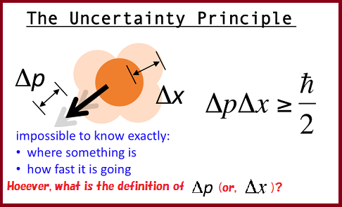
In this section, we shall propose the mathematical formulation ( Theorem 4.15) of Heisenberg's uncertainty principle (Proposition 4.10). Consider the quantum basic structure:
\begin{align}
[{\mathcal C}(H) \subseteq B(H) \subseteq {B(H)}
]
\end{align}
Let $A_i$ $(i=1,2)$ be arbitrary self-adjoint operator on $H$. For example, it may satisfy that
\begin{align}
[A_1 , A_2](:=A_1 A_2 - A_2 A_1 ) =\hbar \sqrt{-1}I
\end{align}
Let ${\mathsf O}_{A_i}=({\mathbb R}, {\cal B}, F_{A_i} )$ be the spectral representation of $A_i$, i.e., $A_i=\int_{\mathbb R} \lambda F_{A_i}( d \lambda )$, which is regarded as the projective observable in $B(H)$. Let $\rho_0= |u\rangle \langle u |$ be a state, where $u \in H$ and $\|u\|=1$. Thus, we have two measurements:
| (B1): | ${\mathsf{M}}_{B(H)} ({\mathsf{O}_{A_1}}{\; :=} ({\mathbb R}, {\cal B}, F_{A_1} ),$ $ S_{[\rho_u]})$ $\qquad \xrightarrow[\scriptsize{\mbox{ expectation}}]{\scriptsize{\mbox{ by (4.17)}}} \langle u, A_1 u \rangle$ |
| (B2): | ${\mathsf{M}}_{B(H)} ({\mathsf{O}_{A_2}}{\; :=} ({\mathbb R}, {\cal B}, F_{A_2} ),$ $ S_{[\rho_u]})$ $\qquad \xrightarrow[\scriptsize{\mbox{ expectation}}]{\scriptsize{\mbox{ by (4.17)}}}\langle u, A_2 u \rangle$
|
\begin{align}
(\forall \rho_u= |u\rangle \langle u | \in {\frak S}^p({\mathcal C}(H)^*))
\end{align}
However, since it is not always assumed that $A_1 A_2 - A_2A_1=0$, we can not expect the existence of the simultaneous observable ${\mathsf{O}_{A_1}}\times {\mathsf{O}_{A_2}}$, namely,
| $\bullet$ | in general, two observables ${\mathsf{O}_{A_1}}$ and ${\mathsf{O}_{A_2}}$ can not be simultaneously measured
|
That is,
| $(B3):$ | the measurement ${\mathsf{M}}_{B(H)} ({\mathsf{O}_{A_1}}\times {\mathsf{O}_{A_2}},$ $ S_{[\rho_u]})$ is impossible, Thus, we have the question:
\begin{align}
\mbox{
Then, what should be done?
}
\end{align}
|
In what follows, we shall answer this.
Let $K$ be another Hilbert space, and let $s$ be in $K$ such that $\| s \|=1$. Thus, we also have two observables ${\mathsf{O}_{A_1 \otimes I}}{\; :=} ({\mathbb R}, {\cal B}, F_{A_1} \otimes I )$ and ${\mathsf{O}_{A_2\otimes I}}{\; :=} ({\mathbb R}, {\cal B}, F_{A_2}\otimes I )$ in the tensor algebra $B(H \otimes K)$.
Put
\begin{align}
\mbox{
the tensor state ${\widehat \rho}_{us}=|u \otimes s \rangle \langle u \otimes s|
$}
\end{align}
And we have the following two measurements:
| $(C_1):$ | ${\mathsf{M}}_{B(H\otimes K)} ({\mathsf{O}_{A_1 \otimes I}},S_{[{\widehat \rho}_{us}]})$ $\qquad \xrightarrow[\scriptsize{\mbox{ expectation}}]{\scriptsize{\mbox{ by (4.17)}}} \langle u, A_1 u \rangle$
|
| $(C_2)$: | ${\mathsf{M}}_{B(H\otimes K)} ({\mathsf{O}_{A_2 \otimes I}},S_{[{\widehat \rho}_{us}]})$ $\qquad \xrightarrow[\scriptsize{\mbox{ expectation}}]{\scriptsize{\mbox{ by (4.17)}}} \langle u, A_1 u \rangle$
|
It is a matter of course that
\begin{align}
\mbox{(C$_1$)=(B$_1$) $\quad$ (C$_2$)=(B$_2$)}
\end{align}
and
| $(C_3)$: | ${\mathsf{M}}_{B(H\otimes K)} ({\mathsf{O}_{A_1\otimes I}}\times {\mathsf{O}_{A_2\otimes I}},$
$ S_{[{\widehat{\rho}_{us}}]})$
is impossible.
|
Thus, overcoming this difficulty, we prepare the following idea:
Preparation 4.11 Let ${\widehat A}_i$ $(i=1,2)$ be arbitrary self-adjoint operator on the tensor Hilbert space $H \otimes K$, where it is assumed that
\begin{align}
[{\widehat A}_1, {\widehat A}_2](:=
{\widehat A}_1{\widehat A}_2- {\widehat A}_2{\widehat A}_1)=0
\quad
\mbox{(i.e.,
the commutativity)}
\tag{4.21}
\end{align}
Let ${\mathsf O}_{{\widehat A}_i}=({\mathbb R}, {\cal B},
F_{{\widehat A}_i} )$ be the spectral representation of ${\widehat A}_i$, i.e.${\widehat A}_i=\int_{\mathbb R} \lambda F_{{\widehat A}_i}
( d \lambda )$, which is regarded as the projective observable in $B(H \otimes K)$. Thus, we have two measurements as follows:
| $(D_1):$ | ${\mathsf{M}}_{B(H\otimes K)} ({\mathsf{O}_{{\widehat A}_1}},S_{[{\widehat \rho}_{us}]})$ $\quad \xrightarrow[\scriptsize{\mbox{ expectation}}]{\scriptsize{\mbox{ by (4.17)}}}\langle u\otimes s,\widehat{A}_1( u\otimes s ) \rangle$
|
| $(D_2)$: | ${\mathsf{M}}_{B(H\otimes K)} ({\mathsf{O}_{{\widehat A}_2}},S_{[{\widehat \rho}_{us}]})$ $\quad \xrightarrow[\scriptsize{\mbox{ expectation}}]{\scriptsize{\mbox{ by (4.17)}}}\langle u\otimes s,\widehat{A}_2( u\otimes s ) \rangle$
|
Note, by the commutative condition (4.21), that the two can be measured by the simultaneous measurement
${\mathsf{M}}_{B(H\otimes K)} ({\mathsf{O}_{{\widehat A}_1}}\times{\mathsf{O}_{{\widehat A}_2}},S_{[{\widehat \rho}_{us}]})$, where ${\mathsf{O}_{{\widehat A}_1}}\times{\mathsf{O}_{{\widehat A}_2}}=({\mathbb R}^2, {\cal B}^2,
F_{{\widehat A}_1} \times F_{{\widehat A}_2} )$.
Again note that any relation between $A_i \otimes I$ and ${\widehat A}_i$ is not assumed. However,
| ${}$ | we want to
regard this simultaneous measurement as the substitute of the above two (C$_1$) and (C$_2$). That is, we want to regard
(D$_1$) and (D$_2$) as the substitute of (C$_1$) and (C$_2$)
|
For this, we have to prepare Hypothesis 4.9 below.
Putting
\begin{align}
{\widehat N}_i := {\widehat A}_i -A_i \otimes I
\quad
(\mbox{and thus, } {\widehat A}_i={\widehat N}_i +A_i \otimes I)
\tag{4.22}
\end{align}
we define the $\Delta_{\widehat{N}_i}^{{\widehat{\rho}_{us}}}$ and ${\overline \Delta}_{\widehat{N}_i}^{{\widehat{\rho}_{us}} }$ such that
\begin{align}
\Delta_{\widehat{N}_i}^{u \otimes s} =& \| {\widehat N}_i (u \otimes s) \|
=
\|
({\widehat A}_i -A_i \otimes I) (u \otimes s )
\|
\tag{4.23}
\\
{\overline \Delta}_{\widehat{N}_i}^{u \otimes s} =&
\| ( {\widehat N}_i - \langle u \otimes s , {\widehat N}_i (u \otimes s)\rangle ) (u \otimes s) \|
\nonumber
\\
=
&
\| ( ({\widehat A}_i -A_i \otimes I) - \langle u \otimes s , ({\widehat A}_i -A_i \otimes I) (u \otimes s)\rangle ) (u \otimes s) \|
\end{align}
where the following inequality:
\begin{align}
\Delta_{\widehat{N}_i}^{{\widehat{\rho}_{us}}}
\ge
{\overline \Delta}_{\widehat{N}_i}^{{\widehat{\rho}_{us}}}
\tag{4.24}
\end{align}
is common sense.
By the commutative condition (4.21), (4.22) implies that
\begin{align}
[{\widehat N}_1,{\widehat N}_2]
+
[{\widehat N}_1, A_2 \otimes I]+[A_1 \otimes I ,{\widehat N}_2]
=
-[A_1 \otimes I, A_2 \otimes I]
\tag{4.25}
\end{align}
Here, we should note that the first term (or, precisely, $
| \langle u \otimes s ,
[\mbox{the first term}] ( u \otimes s) \rangle |
$ ) of (4.25) can be, by the Robertson uncertainty relation (Theorem 4.9), estimated as follows:
\begin{align}
2 {\overline \Delta}_{\widehat{N}_1}^{{\widehat{\rho}_{us}}} \cdot {\overline \Delta}_{\widehat{N}_2}^{{\widehat{\rho}_{us}}}
\ge
| \langle u \otimes s ,
[{\widehat N}_1,{\widehat N}_2] ( u \otimes s) \rangle |
\tag{4.26}
\end{align}
4.3.2.2: Average value coincidence conditions; approximately simultaneous measurement
However, it should be noted that
\begin{align}
\mbox{In the above, any relation between $A_i \otimes I$ and ${\widehat A}_i$ is not assumed.
}
\end{align}
Thus, we think that the following hypothesis is natural.
Hypothesis 4.12 [Average value coincidence conditions ]. We assume that
\begin{align}
&
\langle u \otimes s, {\widehat N}_i(u \otimes s) \rangle =0 \qquad ( \forall u \in H, i=1,2)
\tag{4.27}
\end{align}
or equivalently,
\begin{align}
\langle u \otimes s, {\widehat A}_i(u \otimes s) \rangle
=
\langle u , {A}_i u \rangle
\qquad ( \forall u \in H, i=1,2)
\tag{4.28}
\end{align}
That is,
\begin{align}
&\mbox{the average measured value of ${\mathsf{M}}_{B(H\otimes K)} ({\mathsf{O}_{{\widehat A}_i}},S_{[{\widehat \rho}_{us}]})$}
\\
=
&
\langle u \otimes s, {\widehat A}_i(u \otimes s) \rangle
\\
=
&
\langle u , {A}_i u \rangle
\\
=
&
\mbox{the average measured value of ${\mathsf{M}}_{B(H)} ({\mathsf{O}_{{A}_i}},S_{[{ \rho}_{u}]})$}
\\
&
\quad ( \forall u \in H, ||u||_H =1, i=1,2)
\end{align}
Hence, we have the following definition.
Definition 4.13 [Approximately simultaneous measurement] Let $A_1$ and $A_2$ be (unbounded) self-adjoint operators on a Hilbert space $H$. The quartet $(K, s, \widehat{A}_1, \widehat{A}_2)$ is called an approximately simultaneous observable of $A_1$ and $A_2$, if it satisfied that
| $(E_1):$ | $K$ is a Hilbert space. $s \in K$, $\| s \|_K=1$,$\widehat{A}_1$ and $\widehat{A}_2$ are commutative self-adjoint operators on a tensor Hilbert space $H \otimes K$ that satisfy the average value coincidence condition (4.27), that is,
\begin{align}
\langle u \otimes s, {\widehat A}_i(u \otimes s) \rangle
=
\langle u , {A}_i u \rangle
\qquad ( \forall u \in H, i=1,2)
\tag{4.29}
\end{align}
|
Also,the measurement ${\mathsf{M}}_{B(H\otimes K)} ({\mathsf{O}_{{\widehat A}_1}}\times{\mathsf{O}_{{\widehat A}_2}},S_{[{\widehat \rho}_{us}]})$ is called the approximately simultaneous measurement of ${\mathsf{M}}_{B(H)} ({\mathsf{O}_{A_1}},$ $ S_{[\rho_u]})$ and ${\mathsf{M}}_{B(H)} ({\mathsf{O}_{A_2}},$ $ S_{[\rho_u]})$.
Thus, under the average coincidence condition, we regard
(D$_1$) and (D$_2$) as the substitute of (C$_1$) and (C$_2$)
And
| $(E_2):$ | ${\Delta}_{\widehat{N}_1}^{{\widehat{\rho}_{us}}}$ $(=
\|
(\widehat{A}_1-A_1 \otimes I)(u \otimes s)
\|
)$ and ${ \Delta}_{\widehat{N}_2}^{{\widehat{\rho}_{us}}}$ $(=
\|
(\widehat{A}_2-A_2 \otimes I)(u \otimes s)
\|
)$ are called errors of the approximate simultaneous measurement ${\mathsf{M}}_{B(H\otimes K)} ({\mathsf{O}_{{\widehat A}_1}}\times{\mathsf{O}_{{\widehat A}_2}},S_{[{\widehat \rho}_{us}]})$
|
Lemma 4.14 Let $A_1$ and $A_2$ be (unbounded) self-adjoint operators on a Hilbert space $H$. And let $(K, s, \widehat{A}_1, \widehat{A}_2)$ be an approximately simultaneous observable of
$A_1$ and $A_2$. Then, it holds that
\begin{align}
&
\Delta_{\widehat{N}_i}^{{\widehat{\rho}_{us}}}=
{\overline \Delta}_{\widehat{N}_i}^{{\widehat{\rho}_{us}}}
\tag{4.30}
\\
&
\langle u \otimes s, [{\widehat N}_1, A_2 \otimes I](u \otimes s) \rangle
=
0
\qquad ( \forall u \in H)
\tag{4.31}
\\
&
\langle u \otimes s, [A_1 \otimes I, {\widehat N}_2](u \otimes s) \rangle =0
\quad ( \forall u \in H)
\tag{4.32}
\end{align}
\end{Lemma}
The proof is easy, thus, we omit it.
Under the above preparations, we can easily get "Heisenberg's uncertainty principle" as follows.
\begin{align}
&
{\Delta}_{\widehat{N}_1}^{{\widehat{\rho}_{us}}} \cdot { \Delta}_{\widehat{N}_2}^{{\widehat{\rho}_{us}}}
(=
{\overline \Delta}_{\widehat{N}_1}^{{\widehat{\rho}_{us}}} \cdot {\overline \Delta}_{\widehat{N}_2}^{{\widehat{\rho}_{us}}}
)
\ge
\frac{1}{2}
| \langle u ,
[A_1,A_2] u \rangle |
\quad ( \forall u \in H \mbox{ such that } ||u||=1 )
\tag{4.33}
\end{align}
Summing up, we have the following theorem:
Theorem 4.15 [The mathematical formulation of Heisenberg's uncertainty principle] Let $A_1$ and $A_2$ be (unbounded) self-adjoint operators
on a Hilbert space $H$.
Then. we have the followings:
| $(i):$ | There exists an approximately simultaneous observable $(K, s, \widehat{A}_1, \widehat{A}_2)$ of $A_1$ and $A_2$, that is, $s \in K$, $\| s \|_K=1$,$\widehat{A}_1$ and $\widehat{A}_2$ are commutative self-adjoint operators on a tensor Hilbert space $H \otimes K$ that satisfy the average value coincidence condition (4.27). Therefore, the approximately simultaneous measurement ${\mathsf{M}}_{B(H\otimes K)} ({\mathsf{O}_{{\widehat A}_1}}\times{\mathsf{O}_{{\widehat A}_2}},S_{[{\widehat \rho}_{us}]})$ exists.
|
| $(ii)$: |
And further, we have the following inequality (i.e., Heisenberg's uncertainty principle).
\begin{align}
{\Delta}_{\widehat{N}_1}^{{\widehat{\rho}_{us}}} \cdot { \Delta}_{\widehat{N}_2}^{{\widehat{\rho}_{us}}}
(=
{\overline \Delta}_{\widehat{N}_1}^{{\widehat{\rho}_{us}}} \cdot {\overline \Delta}_{\widehat{N}_2}^{{\widehat{\rho}_{us}}}
)
&
=
\|
(\widehat{A}_1-A_1 \otimes I)(u \otimes s)
\|
\cdot
\|
(\widehat{A}_2-A_2 \otimes I)(u \otimes s)
\|
\nonumber
\\
&
\ge
\frac{1}{2}
| \langle u ,
[A_1,A_2] u \rangle |
\quad ( \forall u \in H \mbox{ such that } ||u||=1 )
\tag{4.34}
\end{align}
|
| $(iii)$: |
In addition, if $A_1 A_2 - A_2 A_1 = \hbar \sqrt{-1}$, we see that
\begin{align}
{\Delta}_{\widehat{N}_1}^{{\widehat{\rho}_{us}}} \cdot { \Delta}_{\widehat{N}_2}^{{\widehat{\rho}_{us}}}
\ge \hbar/2
\quad ( \forall u \in H \mbox{ such that } ||u||=1 )
\tag{4.35}
\end{align}
|
For the proof of (i) and (ii), see
Note that Theorem 4.15 says that
| $(\sharp):$ |
Heisenberg's indeterminacy principle had not been used as "scientific proposition" until 1991.
|
Therefore, we have the following question:
| $(\sharp):$ | Had Heisenberg's indeterminacy principle been used as "scientific proposition"?
|
Now I have a clear answer for this question:
