Let the density functions $f_J$ and $f_A$ be regarded as the probability density functions $f_J$ and $f_A$ such as
Now, let us represent the statements (A) in terms of quantum language: Define the state space $\Omega$ by $\Omega = \{ {\omega}_J , {\omega}_A
\}$ with the discrete metric $d_D$ and the counting measure $\nu$ such that
/
\begin{align}
\nu(\{\omega_J \})=1,
\;\;
\nu(\{\omega_A \})=1
\quad
\end{align}
$\Big(\mbox{It does not matter, even if}
\nu(\{\omega_J \})=a,
\;\;
\nu(\{\omega_A \})=b
\;\;
(a,b >0)
\Big)$. Thus, we have the classical basic structure:
\begin{align}
\mbox{
Classical basic structure$[ C_0(\Omega ) \subseteq L^\infty (\Omega, \nu ) \subseteq B(L^2 (\Omega, \nu ))]$
}
\end{align}
The pure state space is defined by
\begin{align}
{\frak S}^p (C_0(\Omega)^*)= \{ \delta_{\omega_J} , \delta_{\omega_A} \}
\approx
\{ {\omega}_J , {\omega}_A
\}
=
\Omega
\end{align}
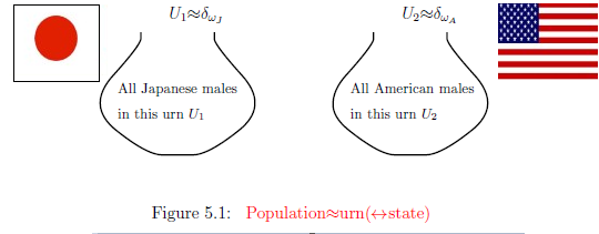
Here, we consider that
\begin{align}
&
\delta_{\omega_J} \quad \cdots \quad
\mbox{"the state of the set $U_1$ of all Japanese males"},
\qquad
\\
&
\delta_{\omega_A} \quad \cdots \quad
\mbox{"the state of the set $U_2$ of all American males"},
\end{align}
and thus, we have the following identification (that is, Figure 5.1):
\begin{align}
U_1 \approx
\delta_{\omega_J}, \qquad
U_2 \approx
\delta_{\omega_A} \quad
\quad
\end{align}
5.1.1 Population(=system) $\leftrightarrow$ paramenter (=state)
Example 5.1 The density functions of the whole Japanese male's height and the whole American male's height is respectively defined by $f_J$ and $f_A$. That is,
\begin{align}
&
\int_\alpha^\beta f_J(x) dx
=
\frac{\mbox{A Japanese male's population whose height is from $\alpha$(cm) to $\beta$(cm)}}{\mbox{A Japanese male's overall population }}
\\
\\
&
\int_\alpha^\beta f_A(x) dx
=
\frac{\mbox{An American male's population whose height is from $\alpha$(cm) to $\beta$(cm)}}{\mbox{An American male's overall population }}
\end{align}
$(A):$ From $
\left[\begin{array}{ll}
\mbox{
the set of all Japanese males
}
\\
\mbox{
the set of all American males
}
\end{array}\right]
$, choose a person (at random). Then, the probability that his height is from $\alpha$(cm) to $\beta$(cm) is given by
\begin{align}
\left[\begin{array}{ll}
[F_{h}([\alpha, \beta))](\omega_J)
=\int_{\alpha}^{\beta} f_J(x) dx
\\
{}
[F_{h}
([\alpha, \beta))](\omega_A)
=\int_\alpha^\beta f_A(x) dx
\end{array}\right]
\end{align}
The observable ${\mathsf O}_{h} = ( {\mathbb R}, {\mathcal B} , F_{h})$ in $L^\infty (\Omega, \nu)$ is already defined by (A). Thus, we have the measurement ${\mathsf M}_{L^\infty (\Omega)} ({\mathsf O}_{h} , S_{ [{}{\delta_{\omega}}]})$ $(\omega \in \Omega =\{\omega_J, \omega_A \})$. The statement (A) is represented in terms of quantum language by
| $(B):$ | The probability that a measured value obtained by the measurement $
\left[\begin{array}{ll}
{\mathsf M}_{{L^\infty (\Omega)}} ({\mathsf O}_{h} ,
S_{ [{}{\omega_J}]})
\\
{\mathsf M}_{{L^\infty (\Omega)}} ({\mathsf O}_{h},
S_{ [{}{\omega_A}]})
\end{array}\right]
$ belongs to an interval $[\alpha, \beta)$ is given by
$ \qquad \qquad \left[\begin{array}{ll} {}_{{{C_0(\Omega) }^*}} \Big( \delta_{\omega_J} , F_{h}([\alpha, \beta) ) \Big){}_{L^\infty (\omega, \nu )} = [F_{h}([\alpha, \beta) )](\omega_J) \\ {}_{{{C_0(\Omega) }^*}} \Big( \delta_{\omega_A} , F_{h}([\alpha, \beta) ) \Big){}_{L^\infty (\omega, \nu )} = [F_{h}([\alpha, \beta) )](\omega_A) \end{array}\right] $ |
5.2.2: Normal observable and student $t$-distribution
Consider the classical basic structure: \begin{align} \mbox{{ $[ C_0(\Omega ) \subseteq L^\infty (\Omega, \nu ) \subseteq B(L^2 (\Omega, \nu ))]$ }} \end{align}where $\Omega = {\mathbb R}$ (=the real line) with the Lebesgue measure $\nu$. Let $\sigma >0$ be a standard deviation, which is assumed to be fixed. Define the measured value space $X$ by ${\mathbb R}$ (i.e., $X={\mathbb R}$). Define the normal observable ${\mathsf O}_{G_\sigma} $ ${{=}}$ $(X(={}{\mathbb R}) , {\cal B}_{{\mathbb R}}^{} , G_{\sigma})$ in $L^\infty ({\Omega}{}, \nu )$ such that
\begin{align} [G_{\sigma}(\Xi) ]( {\omega} ) = \frac{1}{{\sqrt{2 \pi } \sigma}} \int_{\Xi} \exp \left[ {}- \frac{1}{2 \sigma^2 } ({x} - {\omega} )^2 \right] d{x} \tag{5.1} \\ \quad (\forall \Xi \in {\cal B}_{{X}}^{}( ={\cal B}_{{\mathbb R}}^), \; \forall {\omega} \in \Omega (={\mathbb R} )) \end{align} where ${\cal B}_{\mathbb R}$ is the Borel field. For example, \begin{align} & \frac{1}{\sqrt{2 \pi \sigma^2}} \int_{-\sigma}^{\sigma} e^{- \frac{x^2}{2 \sigma^2}} dx =0.683..., \qquad \frac{1}{\sqrt{2 \pi \sigma^2}} \int_{-2 \sigma}^{2 \sigma} e^{- \frac{x^2}{2 \sigma^2}} dx = 0.954..., \nonumber \\ & \frac{1}{\sqrt{2 \pi \sigma^2}} \int_{-1.96 \sigma}^{1.96 \sigma} e^{- \frac{x^2}{2 \sigma^2}} dx {\doteqdot} 0.95 \tag{5.2} \end{align}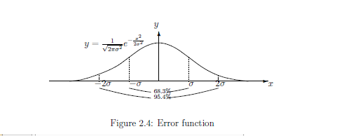
Next, consider the parallel observable $\otimes_{k=1}^n {\mathsf O}_{G_\sigma}$ $=$ $({\mathbb R}^n, {\mathcal B}_{{\mathbb R}^n}, \otimes_{k=1}^n {G_\sigma})$ in $L^\infty (\Omega^n, \nu^{\otimes n})$ and restrict it on
\begin{align} K=\{(\omega , \omega, \ldots, \omega ) \in \Omega^n \;|\; \omega \in \Omega \} (\subseteq \Omega^n) \end{align}This is essentially the same as the simultaneous observable ${\mathsf O}^n$ $=$ $({\mathbb R}^n, {\mathcal B}_{{\mathbb R}^n}, \times_{k=1}^n {G_\sigma})$ in $L^\infty (\Omega)$. That is,
\begin{align} & [(\times_{k=1}^n {G_\sigma})(\Xi_1 \times \Xi_2 \times \cdots \times \Xi_n )](\omega) = \times_{k=1}^n [G_{\sigma}(\Xi_k) ]( {\omega} ) \nonumber \\ = & \times_{k=1}^n \frac{1}{{\sqrt{2 \pi } \sigma}} \int_{\Xi_k} \exp \left[ {}- \frac{1}{2 \sigma^2 } ({x_k} - {\omega} )^2 \right] d{x_k} \tag{5.3} \\ & \quad (\forall \Xi_k \in {\cal B}_{{X}}^{}( ={\cal B}_{{\mathbb R}}^), \; \forall {\omega} \in \Omega (={\mathbb R} )) \end{align} Then, for each $(x_1,x_2, \cdots, x_n )\in X^n (={\mathbb R}^n )$, define \begin{align} & \overline{x}_n = \frac{x_1 + x_2 + \cdots + x_n }{n} \\ & U_n^2 =\frac{(x_1 - \overline{x}_n)^2 + (x_2 - \overline{x}_n)^2+ \cdots +( x_n - \overline{x}_n)^2}{n-1} \end{align} and define the map $\psi:{\mathbb R}^n \to {\mathbb R}$ such that \begin{align} \psi (x_1, x_2, \ldots , x_n ) = \frac{\overline{x}_n - \omega}{U_n / \sqrt{n}} \end{align}Then, we have the observable ${\mathsf O}_{T_n^\sigma} $ ${{=}}$ $(X(={}{\mathbb R}) , {\cal B}_{{\mathbb R}}^{} , T_n^\sigma)$ in $L^\infty ({\mathbb R} )$ such that
\begin{align} [T_n^\sigma (\Xi )](\omega ) = \Big[G_\sigma \Big(\{ ( x_1, x_2,...,x_n ) \in {\mathbb R}^n \;\;|\;\; \frac{\overline{x}_n - \omega }{U_n / \sqrt{n}} \in \Xi \}\Big)\Big](\omega ) \quad (\forall \Xi \in {\mathcal F} ) \tag{5.4} \end{align}The observable ${\mathsf O}_{T_n^\sigma} $ ${{=}}$ $(X(={}{\mathbb R}) , {\cal B}_{{\mathbb R}}^{} , T_n^\sigma)$ in $L^\infty({\mathbb R} )$ is called the student $t$ observable. Here,putting
\begin{align} f_n^\sigma (x)=\frac{\{\Gamma (n/2)}{\sqrt{(n-1)\pi} \Gamma ((n-1)/2)} (1 + \frac{x^2}{n-1})^{-n/2} \qquad \mbox{$( \Gamma$ is Gamma function)} \tag{5.5} \end{align} we see that \begin{align} [T_n^\sigma (\Xi )](\omega ) = \int_{\Xi} f_n^\sigma (x) dx \quad (\forall \Xi \in {\mathcal F} ) \tag{5.6} \end{align}which is independent of $\omega$ and $\sigma$. Also note that
\begin{align} \lim_{n \to \infty } f_n^\sigma (x)=& \lim_{n \to \infty } \frac{\Gamma (n/2)}{\sqrt{(n-1)\pi} \Gamma ((n-1)/2)} (1 + \frac{x^2}{n-1})^{-n/2} \\ = & \frac{1}{\sqrt{2 \pi}} e^{- \frac{x^2}{2}} \end{align}
thus, if $n \ge 30$, it can be regarded as the normal distribution $N(0,1)$( that is,mean $0$,the standard deviation $1$).
