13.2: Regression analysis
Let
$(T{{=}} \{ t_0,t_1,$
$\ldots,$
$ t_N\} , \pi:
T \setminus \{ t_0 \} \to T)$
be a tree.
Let
$\widehat{\mathsf O}_{T{}}$
${{=}} (
\times_{t \in T} X_t, $
${\boxtimes_{t \in T} {\cal F}_t}, $
$
{\widehat F}_{t_0})$
be the realized causal observable
of
a
sequential causal observable
$[{}\{ {\mathsf O}_t \}_{ t \in T} ,
\{ \Phi_{\pi(t), t }{}: $
$L^\infty ({\Omega}_{t})\to L^\infty ({\Omega }_{\pi(t)}) \}_{ t \in T\setminus \{t_0\} }$
$]$.
Consider a
measurement
Assume that
a measured value obtained by the measurement
belongs to
${\widehat \Xi}
\;(\in
{\boxtimes_{t \in T} {\cal F}_t}
)$.
Then,
there is a reason to infer that
The poof is a direct consequence of
Axiom 2 (causality; $\S$10.3)
and
Fisher maximum likelihood method
(Theorem 5.6Theorem in $\S$5.2).
Thus, we omit it.
Now we will answer
Problem 13.1
in terms of quantum language,
that is,
in terms of
regression analysis
(Theorem 13.4).
Let
$(T{{=}}$
$ \{ 0,1,2\} , \pi:
T \setminus \{ 0 \} \to T)$
be the parent map representation of a tree,
where it is assumed that
Put
$\Omega_0
=\{\omega_1, \omega_2,\ldots,\omega_5\}$,
$\Omega_1 = \mbox{interval}
[100,200]$,
$\Omega_2 = \mbox{interval}[30,110]$.
Here, we consider that
For each
$t \;(\in \{ 1,2 \})$,
the deterministic map
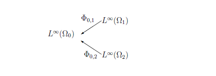
$\phi_{0,t}{}: \Omega_0 \to \Omega_t $
is defined by
$\phi_{0,1}=h$(height function),
$\phi_{0,2}=w$(weight function).
Thus,
for each
$t \;(\in \{ 1,2\})$,
the
deterministic causal operator
$\Phi_{0,t}{}: L^\infty (\Omega_t) \to L^\infty (\Omega_0) $
is defined by
According to
Fisher's maximum likelihood method (Theorem5.6 in $\S$5.2)
and
the existence theorem of the realized causal observable,
we have the following theorem:
It should be noted that
That is,
\begin{align}
&
\fbox{regression analysis}
\\
\\
=
&
\color{blue}{
\color{magenta}{
\underset{\mbox{or, some inference method}}{\fbox{Fisher's maximum likelihho method}}
}
+ \fbox{realized causal observable}
}
\end{align}
$(\sharp):$
regression analysis is related to
both
Axiom 1 (measurement; $\S$2.7)
and
Axiom 2 (causality; $\S$10.3)
Answer 13.5 [(Continued from Problem 13.1 (Inference problem))Regression analysis]

For each $t=1,2$, let ${\mathsf O}_{G_{\sigma_t}} {{=}} ({\mathbb R}, {\cal B}_{\mathbb R}, G_{\sigma_t})$ be the normal observable with a standard deviation $\sigma_t >0$ in $L^\infty (\Omega_t)$. That is,
\begin{align} [G_{\sigma_t}(\Xi)] (\omega) = \frac{1}{\sqrt{2 \pi \sigma_t^2}} \int_{\Xi} e^{- \frac{(x - \omega)^2}{2 \sigma_t^2}} dx \quad (\forall \Xi \in {\cal B}_{\mathbb R}, \forall \omega \in \Omega_t ) \end{align}Thus, we have a deterministic sequence observable $[ \{{\mathsf O}_{G_{\sigma_t}}\}_{t=1,2} , \{ \Phi_{0, t} : L^\infty (\Omega_t) \to L^\infty (\Omega_0)\}_{t=1,2} ]$. Its realization $\widehat{\mathbb O}_{T{}}$ ${{=}}$ $({\mathbb R}^2, {\cal F}_{{\mathbb R}^2}, {\widehat F}_0)$ is defined by
\begin{align} & [{\widehat F}_0(\Xi_1 \times \Xi_2 )] (\omega) = [\Phi_{0,1} G_{\sigma_1} ] (\omega) \cdot [\Phi_{0,2} G_{\sigma_2}] (\omega) = [G_{\sigma_1} ({\Xi_1})] (\phi_{0,1}(\omega)) \cdot [G_{\sigma_2} ({\Xi_2})] (\phi_{0,2}(\omega)) \\ \\ & \qquad \qquad \qquad \qquad (\forall \Xi_1, \Xi_2 \in {\cal B}_{\mathbb R} , \; \forall \omega \in \Omega_0 = \{\omega_1, \omega_2,\ldots,\omega_5\} ) \end{align}Let $N$ be sufficiently large. Define intervals $\Xi_1, \Xi_2 \subset {\mathbb R}$ by
\begin{align} \Xi_1 =\left[{}165 - \frac1{N}, 165 + \frac1{N}\right], \qquad \Xi_2 =\left[{}65 - \frac1{N}, 65+ \frac1{N} \right] \end{align} The measured data obtained by a measurement ${\mathsf M}_{L^\infty (\Omega_0)} (\widehat{\mathbb O}_{T{}}, S_{[\ast]})$ is \begin{align} (165,65) \; (\in {\mathbb R}^2) \end{align}Thus, measured value belongs to $\Xi_1 \times \Xi_2$. Using regression analysis ( Theorem 13.4 ) is characterized as follows:
| $(\sharp):$ | Find $\omega_0$ $(\in \Omega_0)$ such as \begin{align} [{\widehat F}_0(\{\Xi_1 \times \Xi_2)] (\omega_0 ) = \max_{\omega \in \Omega } [{\widehat F}_0(\{\Xi_1 \times \Xi_2)] (\omega ) \end{align} |
Now, let us answer Problem 13.2 in terms of quantum language (or, by using regression analysis (Theorem 13.4).
Answer 13.6 [(Continued from Problem 13.2 (Control problem))Regression analysis]
In Problem 13.2, it is natural to consider that the tree $T=\{0,1,2,3\}$ is discrete time, that is, the linear ordered set with the parent map $\pi :T\setminus\{0\} \to T$ such that $\pi ( t ) = t-1$ $\;(t=1,2,3)$. For example, put
\begin{align} \Omega_0 = [0,\; 1] \times [0,\; 2], \; \Omega_1 =[0,\; 4] \times [0,\; 2], \;\; \Omega_2 = [0,,\; 6] \times [0,\; 2], \;\; \Omega_3 = [0, \; 8] \times [0,\; 2] \end{align}For each $t=1,2,3$, define the deterministic causal map $\phi_{\pi(t),t}{}: \Omega_{\pi(t)} \to \Omega_t $ by (13.3), that is,
\begin{align} & \phi_{0,1}(\omega_0 ) = (\alpha + \beta, \beta) &\quad& (\forall \omega_0 =(\alpha, \beta ) \in \Omega_0 = [0,\; 1] \times [0,\; 2]) \\ & \phi_{1,2 }(\omega_1 ) = (\alpha + \beta, \beta) &\quad& (\forall \omega_1 =(\alpha, \beta ) \in \Omega_1=[0,\; 4] \times [0,\; 2] ) \\ & \phi_{2,3 }(\omega_2 ) = (\alpha + \beta, \beta) &\quad& (\forall \omega_2 =(\alpha, \beta ) \in \Omega_2 =[0,\; 6] \times [0,\; 2] ) \end{align}Thus, we get the deterministic sequence causal map $\{\phi_{\pi(t),t}{}: \Omega_{\pi(t)} \to \Omega_t\}_{t \in \{1,2,3\}}$, and the deterministic sequence causal operator $\{\Phi_{\pi(t),t}{}: L^\infty (\Omega_{t}) \to L^\infty (\Omega_{\pi(t)} ) \}_{t \in \{1,2,3\}}$. That is,
\begin{align} (\Phi_{0,1}f_1)(\omega_0) \!=\! f_1( \phi_{0,1}(\omega_0)) & \quad \; (\forall f_1 \in L^\infty (\Omega_1), \forall \omega_0 \in \Omega_0) \\ (\Phi_{1,2}f_2)(\omega_1) \!=\! f_2( \phi_{1,2}(\omega_1)) & \quad \; ( \forall f_2 \in L^\infty (\Omega_2), \forall \omega_1 \in \Omega_1) \\ (\Phi_{2,3}f_3)(\omega_2) \!=\! f_3( \phi_{2,3}(\omega_2)) & \quad \; ( \forall f_3 \in L^\infty (\Omega_3), \forall \omega_1 \in \Omega_2). \end{align}Illustrating by the diagram, we see
\begin{align} { {\mbox{$ {L^\infty (\Omega_0)} $}} } \mathop{\longleftarrow}^{\Phi_{0, 1 } } {\mbox{$ {L^\infty (\Omega_{1})} $}} \mathop{\longleftarrow}^{\Phi_{1,2 } } {\mbox{$ {L^\infty (\Omega_{2})} $}} \mathop{\longleftarrow}^{\Phi_{2,3 } } {\mbox{$ L^\infty (\Omega_{3}) $}} \end{align}And thus, $\phi_{0,2}(\omega_0)=\phi_{1,2}(\phi_{0,1}(\omega_0))$, $\phi_{0,3}(\omega_0)=\phi_{2,3}(\phi_{1,2}(\phi_{0,1}(\omega_0)))$, Therefore, note that $\Phi_{0,2}=\Phi_{0,1}\cdot \Phi_{1,2}$, $\;\;$ $\Phi_{0,3}=\Phi_{0,1}\cdot \Phi_{1,2} \cdot \Phi_{2,3}$.

Let ${\mathbb R}$ be the set of real numbers. Fix $\sigma>0$. For each $t=0,1,2$, define the normal observable ${\mathsf O}_{t} {{\equiv}} ({\mathbb R}, {\cal B}_{\mathbb R}, G_{\sigma})$ in $L^\infty (\Omega_t)$ such that
\begin{align} & [G_{\sigma}(\Xi)] (\omega_t ) = \frac{1}{\sqrt{2 \pi \sigma^2}} \int_{\Xi} \exp({- \frac{(x - \alpha)^2}{2 \sigma^2}}) dx \\ & (\forall \Xi \in {\cal B}_{\mathbb R}, \forall \omega_t =(\alpha, \beta) \in \Omega_t {{=}} [{}0, \; 2t+2{}]\times [0, \;2]). \end{align}Thus, we have the deterministic sequential causal observable $[ \{{\mathsf O}_{t}\}_{t=1,2,3} , \{\Phi_{\pi(t),t}{}: L^\infty (\Omega_{t}) \to L^\infty (\Omega_{\pi(t)} ) \}_{t \in \{1,2,3\}} ]$. And thus, we have the realized causal observable $\widehat{\mathsf O}_{T{}}$ ${{=}}$ $({\mathbb R}^3, {\cal F}_{{\mathbb R}^3}, {\widehat F}_0)$ in ${L^\infty (\Omega_0)}$ such that ( using Theorem 12.8 )
\begin{align} & [{\widehat F}_0(\Xi_1 \times \Xi_2 \times \Xi_3)] (\omega_0) = \big[ \Phi_{0,1} \big(G_{\sigma} ({\Xi_1}) \Phi_{1,2} (G_{\sigma} ({\Xi_2}) \Phi_{2,3} (G_{\sigma} ({\Xi_3}) )) \big) \big] (\omega_0) \\ = & [\Phi_{0,1} G_{\sigma} ({\Xi_1})] (\omega_0) \cdot [\Phi_{0,2} G_{\sigma}({\Xi_2})] (\omega_0) \cdot [\Phi_{0,3} G_{\sigma}({\Xi_3})] (\omega_0) \\ = & [G_{\sigma} ({\Xi_1})] (\phi_{0,1}(\omega_0)) \cdot [G_{\sigma} ({\Xi_2})] (\phi_{0,2}(\omega_0)) \cdot [G_{\sigma}({\Xi_3})] (\phi_{0,3}(\omega_0)) \\ & \qquad \qquad (\forall \Xi_1, \Xi_2, \Xi_3 \in {\cal B}_{\mathbb R}, \; \forall \omega_0 =(\alpha, \beta) \in \Omega_0 = [0, \; 1] \times [0, \; 2]) \end{align}Our problem (i.e., Problem 13.2Problem}) is as follows,
| $(\sharp_1):$ | Determine the parameter $(\alpha, \beta )$ such that the measured value of ${\mathsf M}_{L^\infty (\Omega_0)} ($ $\widehat{\mathsf O}_{T{}}, $ $S_{[\ast]})$ is equal to $(1.9, 3.0, 4.7)$ |
For a sufficiently large natural number
$N$,
put
| $(\sharp_2):$ | Find $(\alpha, \beta)$ $(=\omega_0 \in \Omega_0)$ such that \begin{align} [{\widehat F}_0(\Xi_1 \times \Xi_2 \times \Xi_3 )] (\alpha, \beta) = \max_{ (\alpha, \beta )} [{\widehat F}_0(\Xi_1 \times \Xi_2 \times \Xi_3 )] \end{align} |
( $ \frac{\partial}{\partial \alpha}\{\cdots \}=0, \frac{\partial}{\partial \beta}\{ \cdots \}=0 \mbox{ and thus,} $ ) \begin{align} \Longrightarrow & \left\{\begin{array}{ll} (1.9 -(\alpha + \beta)) + (3.0 - (\alpha + 2 \beta)) + (4.7 - (\alpha + 3 \beta)) = 0 \\ (1.9 -(\alpha + \beta)) + 2 (3.0 - (\alpha + 2 \beta)) + 3 (4.7 - (\alpha + 3 \beta)) = 0 \end{array}\right. \\ \Longrightarrow & \quad (\alpha, \beta) = (0.4, 1.4) \end{align} Therefore, in order to obtain a measured value $(1.9, \; 3.0, \; 4.7)$, it suffices to put \begin{align} (\alpha, \beta) =(0.4, \; 1.4) \end{align} Remark 13.7 For completeness, note that,
| $\bullet$ |
From the theoretical point of view,
|

