16.1: Bayes=Kalman method (in $L^\infty(\Omega, m)$)
Recall
Theorem 9.11 (Bayes' theorem),
which will be generalized
as Bayes=Kalman operator
as follows.
Let
$t_0$
be the root
of a tree $T$.
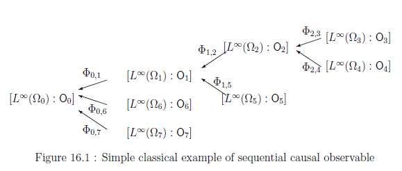
For each $t \in T$, consider the classical basic structure:
Let
$[{\mathbb O}_T{}]$
$=$
$[{}
\{ {\mathsf{O}}_t (\equiv (X_t ,$
$ {\cal F}_{t} , {F}_t ))
\}_{ t \in T} ,
\{ \Phi^{t_1,t_2}{}: $
$L^\infty (\Omega_{t_2}) \to L^\infty (\Omega_{t_1}) \}_{(t_1,t_2) \in T^2_\le }$
$]$
be
a sequential causal observable
with
the realization
$\widehat{\mathsf{O}}_{t_0} $
$\equiv$
$(\times_{t \in T } X_t , $
$\boxtimes_{t \in T } {\cal G}_t,$
${\widehat F}_{t_0})$
in $L^\infty (\Omega_{t_0})$.
For example,

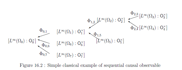
For each $t \in T$, consider another observable ${\mathsf O}_t'=( Y_t, {\mathcal G}_t, G_t)$ in $L^\infty(\Omega_t, m_t )$, and the simultaneous observable ${\mathsf O} \times {\mathsf O}_t'=( X_t \times Y_t, {\mathcal F}_t \boxtimes {\mathcal G}_t, F_t \times G_t)$ in $L^\infty(\Omega_t, m_t )$. And let $[{\mathbb O}_T^\times{}]$ $=$ $[{} \{ {\mathsf{O}}_t^\times (\equiv (X_t \times Y_t ,$ $ {\cal F}_{t} \boxtimes {\cal G}_t , {F}_t \times G_t )) \}_{ t \in T} , \{ \Phi^{t_1,t_2}{}: $ $L^\infty (\Omega_{t_2}) \to L^\infty (\Omega_{t_1}) \}_{(t_1,t_2) \in T^2_\le }$ $]$ be a sequential causal observable with the realization $\widehat{\mathsf{O}}_{t_0}^\times $ $\equiv$ $(\times_{t \in T } (X_t \times Y_t) , $ $\boxtimes_{t \in T } ({\cal F}_{t} \boxtimes {\cal G}_t),$ ${\widehat H}_{t_0})$ in $L^\infty (\Omega_{t_0})$.
For example,

Thus we have the mixed measurement ${\mathsf M}_{L^\infty (\Omega_{t_0})} (\widehat{\mathsf{O}}_{t_0}^\times, \overline{S}_{[\ast]}({{z}}_0 ) )$, where ${{z}}_0 \in L^1_{+1} (\Omega_{t_0} )$. Assume that we know that the measured value $(x,y)$ $( = ( (x_t)_{t\in T}, (y_t)_{t\in T}, ) \in (\times_{t \in T} X_t) \times (\times_{t \in T} Y_t) )$ obtained by the measurement ${\mathsf M}_{L^\infty (\Omega_{t_0})} (\widehat{\mathsf{O}}_{t_0}^\times, \overline{S}_{[\ast]}({{z}}_0 ) )$ belongs to $(\times_{t \in T} \Xi_t) \times $ $ (\times_{t \in T}Y_t) \;$ $(\in (\boxtimes_{t \in T}{\mathcal F}_t) \boxtimes (\boxtimes_{t \in T} {\mathcal G}_t) )$. Then, by Axiom${}^{{ (m)}}$ 1($\S$9.1), we can infer that
| $(A):$ | the probability $ P_{\times_{t \in T} \Xi_t} ( (G_t (\Gamma_t))_{t \in T} ) $ that $y$ belongs to $\times_{t \in T} \Gamma_t (\in \boxtimes_{t \in T} {\cal G}_t)$ is given by \begin{align} & P_{\times_{t \in T} \Xi_t} ( (G_t (\Gamma_t))_{t \in T} ) \nonumber \\ = & \frac{\int_{\Omega_0} [ {\widehat H}_{t_0} ( (\times_{t \in T} \Xi_t) \times (\times_{t \in T} \Gamma_t) ) ] (\omega_0) \; {{z}}_0 (\omega_0 ) \; m_0 (d \omega_0) }{ \int_{\Omega_0} [ {\widehat H}_{t_0} (\times_{t \in T} \Xi_t) \times (\times_{t \in T}Y_t) ](\omega_0) \; {{z}}_0 (\omega_0 ) \; m_0(d \omega_0 )} \tag{16.1} \\ & \quad (\forall \Gamma_t \in {\cal G}_t, t \in T). \nonumber \end{align} |
Thus, putting ${\widehat P}_{\times_{t \in T} \Xi_t} ( G_s (\Gamma_s) )=P_{\times_{t \in T} \Xi_t} ( (G_t (\Gamma_t))_{t \in T} )$, we see that $ {\widehat P}_{\times_{t \in T} \Xi_t} \in L^1_{+1}(\Omega_s, m_s ) $. That is, there uniquely exists $ {{z}}_s^a \in L^1_{+1} (\Omega_s , m_s) $ such that
\begin{align} & {\widehat P}_{\times_{t \in T} \Xi_t} ( (G_s (\Gamma_s)) = {}_{{}_{L^1(\Omega_s)}} \langle {{z}}_s^a, G_s (\Gamma_s) \rangle {}_{{}_{L^\infty(\Omega_s)}} = \int_{\Omega_s} [G_s (\Gamma_s)](\omega_s ) {{z}}_s^a(\omega_s ) m_s ( d \omega_s ) \nonumber \end{align}for any observable $(Y_s, {\cal G}_s, G_s)$ in $L^\infty (\Omega_s)$. That is because the linear functional ${\widehat P}_{\times_{t \in T} \Xi_t} : L^\infty(\Omega_s ) \to {\mathbb C} $ (complex numbers) is weak$^*$ continuous. After all,
| $(B):$ | we can define the Bayes-Kalman operator $[B_{\widehat{\mathsf{O}}_{t_0} }^s(\times_{t \in T} \Xi_t)]: L^1_{+1}(\Omega_{t_0})$ $ \to L^1_{+1}( \Omega_s)$ such that \begin{align} \quad \overset{\mbox{(pretest state)}}{ \underset{ (\in L^1_{+1}(\Omega_{t_0}))} {\fbox{$ {{{z}}_0} $ }} } \xrightarrow[\scriptsize{\mbox{Bayes-Kalman operator}}]{\mbox{ $\qquad [B_{\widehat{\mathsf{O}}_{t_0} }^s(\times_{t \in T} \Xi_t)] \qquad$}} \overset{\mbox{(posttest state)}}{ \underset{( \in L^1_{+1}(\Omega_s))} {\fbox{$ {{{z}}_s^a} $ }} } \tag{16.2} \end{align} |
which is the generalization of the Bayes operator (9.5).
Remark 16.1 We have frequently discussed the Bayes=Kalman filter, for example, in ref. [8] in $\S$0.0. However, these arguments are too theoretical. In this chapter, we devote ourselves to the numerical aspect of the Kalman filter.
