17.1: Equilibrium statistical mechanical phenomena
concerning Axiom 2
(causality)
Equilibrium statistical mechanical phenomena
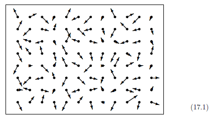
In Newtonian mechanics, any state of a system composed of
$N ({}\approx 10^{24}{})$ particles is represented by a point
$({}q , p{})$
$\bigl(\equiv$
(position, momentum)
$=
$
$({} q_{1n}, q_{2n}, q_{3n} ,$
$ p_{1n} , p_{2n} ,$
$ p_{3n}{})_{n=1}^N $
$\bigl)$
in
a phase
(or state) space
${\mathbb R}^{6N}$.
Let ${\cal H}: {\mathbb R}^{6N} \to {\mathbb R}$
be a Hamiltonian
such that
Fix a positive $E>0$.
And define
the measure
$\nu_{{}_E} $
on
the energy surface
${{\Omega}}_{{}_E}$
($\equiv$
$\{ ({}q, p{}) \in {\mathbb R}^{6N}{}
\; | \;
{\cal H}({}q,p{}) = E \}$)
such that
and
$d m_{6N-1}$
is
the usual surface Lebesgue measure on
${{\Omega}}_{{}_E} $.
Let
$\{ {{{}} \psi}^{{}_E}_t \}_{ - \infty < t < \infty }$
be the flow
on
the energy surface
${{\Omega}}_{{}_E}$
induced by
the
Newton equation
with the Hamiltonian
${\cal H}$,
or equivalently,
Hamilton's canonical equation:
Liouville's theorem
says that
the measure
${ \nu}_{{}_E}$
is
invariant concerning
the flow
$\{ {{{}} \psi}^{{}_E}_t \}_{ - \infty < t < \infty }$.
Defining the normalized measure
$ {\overline \nu}_{{}_E}$
such that
${\overline \nu}_{{}_E}$
$=$
$\frac{ { \nu}_{{}_E} }{ { \nu}_{{}_E} ({}{{\Omega}}_{{}_E}{}) }$,
we have the
normalized measure space
$({}{{\Omega}}_{{}_E} , {\cal B }_{{{\Omega}}_{{}_E} } ,
{\overline \nu}_{{}_E} {})$.
Putting
${\cal A}=C_0(\Omega_{{}_E})$
$=C(\Omega_{{}_E})$
(from the compactness of $\Omega_{{}_E}$),
we have the classical basic structure:
Thus, putting
$T={\mathbb R}$,
and solving the (17.3),
we get
$\omega_t =
(q(t),p(t))$,
$\phi_{t_1.t_2} = \psi_{t_2 -t_1}^E$,
$\Phi^*_{t_1. t_2 } \delta_{\omega_{t_1}}
=
\delta_{\phi_{t_1. t_2} (\omega_{t_1} )}
$
$(\forall \omega_{t_1} \in \Omega_{{}_E})$,
and further we define
the sequential deterministic causal operator
$\{\Phi_{t_1, t_2 }: L^\infty (\Omega_{{}_E}) \to
L^\infty (\Omega_{{}_E})
\}_{(t_1.t_2) \in T_{\le}^2}$.
Now let us begin with
the well-known ergodic theorem.
For
example,
consider one particle
$P_1$.
Put
Clearly, it holds that
$S_{P_1} \subsetneq \Omega_{{}_E}$.
Also,
if
$\psi^{{}_E}_t (
S_{P_1}
) \subseteq
S_{P_1}
$
$(0 {{\; \leqq \;}}\forall t < \infty )$,
then
the particle $P_1$
must always stay a corner.
This contradicts
②
Therefore,
②
means the following:
The ergodic theorem
says that
the above
②$'$
is equivalent to the following equality:
After all,
the ergodic property ②$'$
($\Leftrightarrow$ (17.4)
)
says that
if
$T$
is sufficiently large,
it holds that
Put
${\overline m}_{{}_T}(dt) = \frac{dt}{T}$.
The probability space
$([\alpha, \alpha+ T], {\cal B}_{[\alpha, \alpha + T]}, {\overline m}_{{}_T})$
(or equivalently,
$([0,T], {\cal B}_{[0,T]},$
$ {\overline m}_{{}_T})$
)
is called
a (normalized)
first staying time space,
also,
the probability space
$({}{{\Omega}}_{{}_E} , {\cal B}_{ {{\Omega}}_{{}_E} } , {\overline \nu}_{{}_E} {})$
is called
a
(normalized)
second staying time space.
Note that
these mathematical probability spaces
are not related to
"probability".
Put
$K_N = \{ 1,2,\ldots, N ({}{{\approx}} 10^{24}{}) \} $.
For each
$k$
$({}\in K_N )$,
define the coordinate map
${\pi}_k{}: {{\Omega}}_{{}_E} ({}\subset {\mathbb{R}}^{6N}{}) \to {\mathbb{R}}^6 $
such that
for all
$
\omega=
(q,p)$
$=$
$({} q_{1n},$
$ q_{2n},$
$ q_{3n} ,$
$ p_{1n} ,$
$ p_{2n} , p_{3n}{})_{n=1}^N $
$\in$
$ {{\Omega}}_{{}_E} ({}\subset {\mathbb{R}}^{6N}{})$.
Also,
for any subset
$K$
$({}\subseteq K_N {{=}}$
$ \{1,2,$
$\ldots,N$
$ ({}{{\approx}} 10^{24}{}) \}{})$,
define the distribution map
$D_{K}^{({}\cdot{})} $
$:
{{\Omega}}_{{}_E} $
$({}\subset {\mathbb{R}}^{6 N}{}) $
$ \to {\cal M}_{+1}^m ({}{\mathbb{R}}^6{}) $
such that
where
${\sharp [{}K] }$
is the number of the elements
of the set $K$.
Let
$\omega_0 (
\in \Omega_{{}_E})
$
be a state.
For each
$n$
$(\in K_N )$,
we define the map
$X_n^{\omega_0}: [0, T] \to {\mathbb R}^6$
such that
And,
we regard
$\{X_n^{\omega_0}\}_{n=1}^N$
as
random variables
(i.e.,
measurable functions
) on
the probability space
$([0,T], {\cal B}_{[0,T]}, {\overline m}_{{}_T})$.
Then,
③
and
④
respectively
means
For example,
as one of typical cases,
consider the motion of $10^{24}$ particles in a cubic box
(whose long side is 0.3m).
It is usual to consider that
"averaging velocity"=$5\times10^{2} {\rm m}/{\rm s}$,
"mean free path"=$10^{-7}{\rm m}$.
And therefore,
the collisions rarely happen
among $\sharp[{}K_0{}]$ particles
in the time interval
$[0, T]$,
and therefore,
the motion is {\lq\lq}almost independent".
For example,
putting $\sharp[{}K_0{}]=10^{10}$,
we can calculate
the number of times
a certain particle collides
with $K_0$-particles
in [0,T]
as
$(10^{-7} \times \frac{10^{24}}{10^{10}})^{-1}
\times {(5 \times 10^2)} \times T$
$\approx 5 \times 10^{-5} \times T$.
Hence,
in order to
expect that
\textcircled{\scriptsize 3}$'$
and
\textcircled{\scriptsize 4}$'$
hold,
it suffices to
consider that
$T
\approx
5$ seconds.
Also, we see, by (17.7) and (17.5), that,
for
$K_0 (\subseteq K_N)$
such that
$1 \le
\sharp[{}K_0{}] \ll N{}
$,
Put
$K_N$
$=$
$\{ 1,2,$
$\ldots,$
$N ( {{\approx}} 10^{24}) \}$.
Let
${\cal H} $,
$E$,
${\nu_{{}_E}}$,
${\overline \nu}_{{}_E}$,
${\pi}_k:{{\Omega}}_{{}_E} \to {\mathbb{R}}^6$
be as in the above.
Then,
summing up
③
and
④,
by (17.7) we have:
Also,
a state
$(q,p) (\in \Omega_{{}_E})$
is called
an
equilibrium state
,
if it satisfies
$D_{K_N}^{ ({}q , p {})} {{\approx}} \rho_{{}_E}$.
Now,
we have the following theorem:
Assume
Hypothesis 17.3
$($
or
equivalently,
③
and
④
$)$.
Then,
for any
$\omega_0 = (q(0), p(0))
\in
\Omega_{{}_E}$,
it holds that
for almost
all
$t$.
That is,
$0 {{\; \leqq \;}}$
${\overline m}_{{}_T}(\{t \in [0,T] : \mbox{(17.12) does not hold}\}$
$\ll 1$.
Proof.
Let
$K_0 \subset K_N$
such that
$1 \ll
\sharp[{}K_0{}]
\equiv N_0
\ll N{}
$
(that is,
$\frac{1}{\sharp[{}K_0{}] } {\approx} 0 {\approx} \frac{\sharp[{}K_0{}] }{N}$
).
Then,
from
Hypothesis 17.3,
the law of large numbers
says that
for almost all time $t$.
Consider the decomposition
$K_N$
$=$
$\{ K_{ ({}1{})} , K_{ (2 {})} ,\ldots,$
$ K_{ (L {})} \}$.
(i.e.,
$K_N=\bigcup_{l=1}^L K_{(l)}$,
$K_{(l)} \cap K_{(l')}=\emptyset
\;\;
(l \not= l')
$
),
where
$\sharp [{}K_{ ({}l{})} {}] {{\approx}} N_0 $
$({}l=1,2,\ldots, L{})$.
From
(7.13),
it holds that,
for each
$k$
$({}= 1,2,\ldots,N $
$({}{{\approx}} 10^{24}{}){})$,
for almost all time $t$.
Thus, by (17.10),
we get (17.12).
Hence, the proof is completed.
We believe that
Theorem 17.4 is just what should be represented by the
"ergodic hypothesis"
such that
Thus, we can assert that
the ergodic hypothesis is related to
equilibrium statistical mechanics.
Here, the ergodic property
②$'$
(or equivalently,
equality (17.5)
and
the above
ergodic hypothesis
should not be confused.
Also, it should be noted that
the ergodic hypothesis does not hold
if the box
( containing particles )
is too large.
The entropy
$H(q,p)$
of a state
$(q,p)
(\in \Omega_{{}_E})
$
is defined by
Since
almost every state
in $\Omega_{{}_E}$
is
equilibrium,
the entropy of
almost every
state
is equal
$k \log \nu_{{}_E}(\Omega_{{}_E})$.
Therefore,
it is natural to assume that
the law of increasing entropy
holds.
Hypothesis 17.1
[Equilibrium statistical mechanical hypothesis].
Assume that about $N ({{\approx}} 10^{24} \approx 6.02 \times 10^{23}$
$\approx$ "the Avogadro constant") particles
(for example,
hydrogen molecules)
move in a box with about $20$ liters.
It is natural
to
assume the following
phenomena
①
$
\text{--}
$
④
①
Every particle obeys Newtonian mechanics.
②
Every particle moves uniformly in the box.
For example,
a particle does not halt in a corner.
③
Every particle moves with the same statistical behavior
concerning time.
④
The motions of particles are $($approximately$)$ independent of each other.
In what follows
we shall
devote ourselves to the problem:
(D)
how to describe
the above
equilibrium statistical mechanical
phenomena
①-④
in terms of quantum language ( =measurement theory).
17.1.2: About ①
17.1.3: About ②
②'
[Ergodic property]:
If
a compact set
$
S(\subseteq \Omega_{{}_E},
S \not= \emptyset )$
satisfies
$\psi^{{}_E}_t (S) \subseteq S$
$(0 {{\; \leqq \;}}\forall t < \infty )$,
then
it holds that
$S=\Omega_{{}_E}$.
17.1.4: About ③ and ④
③'
$\{X_n^{\omega_0}\}_{n=1}^N$
is a
sequence with the
approximately
identical distribution
concerning time.
In other words,
there exists
a normalized measure
$\rho_{{}_E}$
on ${\mathbb R}^6$
$(${}i.e.,
$\rho_{{}_E} \in {\cal M}^m_{+1} ({}{\mathbb R}^6{})${}$)$
such that:
\begin{align}
&
{\overline m}_{{}_T}( \{ t \in [0,T] \;: \; X_n^{\omega_0} ( t) \in \Xi \} )
{{\approx \;}}
\rho_{{}_E}(\Xi )
\label{eq'178}
\\
&
\quad
(\forall \Xi \in {\cal B}_{{\mathbb R}^6}, n=1,2,\ldots, N)
\nonumber
\end{align}
Here,
we can assert the advantage of our method
in comparison with Ruelle's method
as follows.
④$'$
$\{X_n^{\omega_0}\}_{n=1}^N$
is
approximately independent,
in the sense that,
for
any
$
K_0 \subset \{ 1,2,$
$\ldots,$
$N ({}{{\approx}} 10^{24}{})\}
$
such that
$1 {{\; \leqq \;}}
\sharp[{}K_0{}] \ll N{}
$
(
that is,
$\frac{\sharp[{}K_0{}] }{N}
{\approx} 0
$
),
it holds that
\begin{align*}
&
{\overline m}_{{}_T}(
\{
t
\in [0,T]
:
X_{k}^{\omega_0} ( t) \in \Xi_{k} (\in {\cal B}_{{\mathbb R}^{6}} ),
{k} \in K_0 \})
\\
{{\approx}}
&
{\Large \times}_{{k} \in K_0 } {\overline m}_{{}_T}(
\{
t
\in [0,T]
:
X_{k}^{\omega_0} ( t) \in \Xi_{k} (\in
{\cal B}_{{\mathbb R}^{6}}
) \}).
\end{align*}
(E)
$\{ {\pi}_k:\Omega_{{}_E} \to {\mathbb{R}}^6 \}_{k=1}^N$
is approximately
independent random variables
with the identical distribution
in the sense that
there exists $\rho_{{}_E}$
$(\in {\cal M}_{+1}^m ({\mathbb{R}}^6))$
such that
\begin{align}
\bigotimes_{ k \in K_0 }
{\rho_{{}_E}}
(=\text{"product measure"})
{{\approx}}
&
\;
{\overline \nu}_{{}_E}
\circ
({} ({}{\pi}_k{})_{ k \in K_0 }{})^{-1}.
\label{eq'1711}
\end{align}
for all
$K_0 \subset
K_N
$
and
$1 {{\; \leqq \;}}
$
$
\sharp[{}K_0{}] $
$\ll N{}
$.
17.1: Equilibrium statistical mechanical phenomena concerning Axiom 2 (causality)
This web-site is the html version of "Linguistic Copehagen interpretation of quantum mechanics; Quantum language [Ver. 4]" (by Shiro Ishikawa; [home page] )
PDF download : KSTS/RR-18/002 (Research Report in Dept. Math, Keio Univ. 2018, 464 pages)
Remark 17.2
[About the time interval $[0,T]$].
Hypothesis 17.3
[③
and
④
].
17.1.5. Ergodic Hypothesis
