‚±‚МђЯ‚Е‚НЃAѓnѓCѓ[ѓ“ѓxѓ‹ѓO‚М•sЉm’иђ«Њґ—ќ‚Мђ”Љw“I’иЋ®‰»‚рЋ¦‚·ЃB
4.3.2: ѓnѓCѓ[ѓ“ѓxѓ‹ѓO‚М•sЉm’иђ«Њґ—ќ‚Мђ”Љw“I’иЋ®‰»
4.3.2.1 ЏЂ”х
Љо–{Ќ\‘ў
$[{\mathcal C}(H)Ѓ@\subseteq B(H)]_{B(H)}$
‚рЌl‚¦‚й.
$A_i$ $(i=1,2)$‚рѓqѓ‹ѓxѓ‹ѓg‹уЉФ$H$Џг‚М”C€У‚М(”с—LЉE)Ћ©ЊИ‹¤–рЌм—p‘f‚Ж‚·‚й. Ѓ@‚Ѕ‚Ж‚¦‚О, ђіЏЂЊрЉ·ЉЦЊW$[A_1 , A_2](:=A_1 A_2 - A_2 A_1 ) =\hbar \sqrt{-1}I$‚р–ћ‚Ѕ‚·‚Ж‰ј’и‚µ‚Д‚а‚ж‚ў.
ЋАЋІ${\mathbb R}$‚Ж‚»‚Мѓ{Ѓ[ѓЊѓ‹ЏWЌ‡‘М${\cal B}_{\mathbb R} $‚рЌl‚¦‚й.
Ћ©ЊИ‹¤–рЌм—p‘f$A_i$‚МѓXѓyѓNѓgѓ‹•Є‰р$A_i=\int_{\mathbb R} \lambda F_{A_i}( d \lambda )$‚рЋg‚Б‚Д, ЋЛ‰eЉП‘Є—К${\mathsf O}_{A_i}=({\mathbb R}, {\cal B}, F_{A_i} )$ ‚р’и‚Я‚й.
Ћџ‚М“с‚В‚М‘Є’и‚р
“ЇЋћ‘Є’и
‚µ‚Ѕ‚ў.
| $(B_1):$ |
${\mathsf{M}}_{B(H)} ({\mathsf{O}_{A_1}}{\; :=} ({\mathbb R}, {\cal B}, F_{A_1} ),$
$ S_{[\rho_u]})$
$\qquad \xrightarrow[Љъ‘Т’l]{}\langle u, A_1 u \rangle$
\item[(B$_2$)]${\mathsf{M}}_{B(H)} ({\mathsf{O}_{A_2}}{\; :=} ({\mathbb R}, {\cal B}, F_{A_2} ),$
$ S_{[\rho_u]})$
$\qquad \xrightarrow[Љъ‘Т’l]{}\langle u, A_2 u \rangle$
|
\begin{align*}
(\forall \rho_u= |u\rangle \langle u | \in {\frak S}^p({\mathcal C}(H)^*))\end{align*}
‚µ‚©‚µ‚И‚Є‚з,
$A_1 A_2 - A_2A_1=0$‚Ж‚НЊА‚з‚И‚ў‚М‚ЕЃi‚·‚И‚н‚ї,
“с‚В‚МЋЛ‰eЉП‘Є—К${\mathsf O}_{A_1}$‚Ж${\mathsf O}_{A_2}$‚Н‰ВЉ·‚Ж‚Н‰ј’и‚µ‚Д‚ў‚И‚ў‚М‚Е), “ЇЋћЉП‘Є—К${\mathsf{O}_{A_1}}\times {\mathsf{O}_{A_2}}$‚М‘¶ЌЭ‚НЉъ‘Т‚Е‚«‚И‚ў‚М‚Е,
-
€к”К‚Й‚Н,‚±‚М“с‚В‚М‘Є’и‚р“ЇЋћ‘Є’и‚·‚й‚±‚Ж‚Н‚Е‚«‚И‚ў
‚·‚И‚н‚ї,
| $(B_2):$ |
${\mathsf{M}}_{B(H)} ({\mathsf{O}_{A_1}}\times {\mathsf{O}_{A_2}},$
$ S_{[\rho_u]})$
‚Н•s‰В‚Ж‚И‚й.Ѓ@‚»‚¤‚И‚з‚О,
|
‚Е‚ ‚й.
‚±‚М‚Ѕ‚Я‚Й, Џг‚М“с‚В‚М‘Є’и‚рЋџ‚М‚ж‚¤‚ЙЊѕ‚ўЉ·‚¦‚悤.
‚а‚¤€к‚В‚М•К‚Мѓqѓ‹ѓxѓ‹ѓg‹уЉФ$K$‚рЌl‚¦‚Д, $s(\in K)$‚р$\| s \|=1$‚̂悤‚Й‚Ж‚й.
‚Ь‚Ѕ, $B(H \otimes K)$“а‚М“с‚В‚МЉП‘Є—К${\mathsf{O}_{A_1 \otimes I}}{\; :=} ({\mathbb R}, {\cal B}, F_{A_1} \otimes I )$‚Ж${\mathsf{O}_{A_2\otimes I}}{\; :=} ({\mathbb R}, {\cal B}, F_{A_2}\otimes I )$‚рЌl‚¦‚й. Ѓ@‚Ь‚Ѕ, Џу‘Ф‚р
\begin{align*}
\textcolor{red}{\bf
\mbox{
Џу‘Ф${\widehat \rho}_{us}=|u \otimes s \rangle \langle u \otimes s|$}}
\end{align*}
‚Ж’и‚Я‚Д, Ћџ‚М“с‚В‚М‘Є’и‚рЌl‚¦‚й.
| $(C_1):$ |
${\mathsf{M}}_{B(H\otimes K)} ({\mathsf{O}_{A_1 \otimes I}},S_{[{\widehat \rho}_{us}]})$
$\qquad \xrightarrow[Љъ‘Т’l]{}\langle u\otimes s,( A_1 \otimes I)( u\otimes s ) \rangle= \langle u, A_1 u \rangle$
|
| $(C_2):$ |
${\mathsf{M}}_{B(H\otimes K)} ({\mathsf{O}_{A_2 \otimes I}},S_{[{\widehat \rho}_{us}]})$
$\qquad \xrightarrow[Љъ‘Т’l]{}\langle u\otimes s,( A_2 \otimes I)( u\otimes s ) \rangle=\langle u, A_2 u \rangle$
|
“–‘R‚М‚±‚Ж‚Е‚ ‚й‚Є, ‚±‚М“с‚В‚Н‚»‚к‚ј‚кЏг‚М“с‚В‚М(B$_1$)‚Ж(B$_2$)‚Ж“Ї‚¶‚ЖЊ©‚И‚№‚й.
‚·‚И‚н‚ї,
\begin{align*}
\mbox{(C$_1$)=(B$_1$) $\quad$ (C$_2$)=(B$_2$)}
\end{align*}
‚Е‚ ‚й.
‚µ‚Ѕ‚Є‚Б‚Д(‚Ь‚Ѕ‚Н, ${\mathsf{O}_{A_1 \otimes I}}$‚Ж${\mathsf{O}_{A_1 \otimes I}}$‚Н€к”К‚Й‚Н‰ВЉ·‚Е‚И‚ў‚М‚Е), Џг‚М“с‚В‚М‘Є’и‚р“ЇЋћ‘Є’и‚·‚й‚±‚Ж‚Н‚Е‚«‚И‚ў.
‚µ‚Ѕ‚Є‚Б‚Д,‰Ѕ‚Мђi“W‚а‚И‚©‚Б‚Ѕ‚н‚Ї‚Е,
| $(C_3):$ |
${\mathsf{M}}_{B(H\otimes K)} ({\mathsf{O}_{A_1\otimes I}}\times {\mathsf{O}_{A_2\otimes I}},$
$ S_{[{\widehat{\rho}_{us}}]})$
‚Н•s‰В‚Ж‚И‚й.Ѓ@‚»‚¤‚И‚з‚О,Ѓ@
|
‚±‚к‚рђi“W‚і‚№‚й‚Ѕ‚Я‚Й, €И‰є‚̂悤‚ИЌH•v‚р‚µ‚Д,
-
Ѓu${A_1\otimes I}$‚Ж${A_2\otimes I}$‚М“ЇЋћ‘Є’и‚а‚З‚«${\widehat A}_1$‚Ж${\widehat A}_2$Ѓv
‚рЌl‚¦‚й.
ЏЂ”х 4.11
${\widehat A}_i$ $(i=1,2)$‚рѓeѓ“ѓ\ѓ‹ ѓqѓ‹ѓxѓ‹ѓg‹уЉФ$H \otimes K$Џг‚М
”C€У‚М‰ВЉ·‚ИЋ©ЊИ‹¤–рЌм—p‘f‚Ж‚·‚й. ‚·‚И‚н‚ї,
\begin{align}
[{\widehat A}_1, {\widehat A}_2](:=
{\widehat A}_1{\widehat A}_2- {\widehat A}_2{\widehat A}_1)=0
\tag{4.21}
\end{align}
‚Ж‚·‚й.
${\widehat A}_i$‚МѓXѓyѓNѓgѓ‹•\Њ»${\widehat A}_i=\int_{\mathbb R} \lambda F_{{\widehat A}_i}( d \lambda )$‚рЋg‚Б‚Д,Ѓ@$B(H \otimes K)$“а‚МЉП‘Є—К${\mathsf O}_{{\widehat A}_i}=({\mathbb R}, {\cal B},
F_{{\widehat A}_i} )$‚р’и‚Я‚й.
‚±‚±‚Е, Ћџ‚М“с‚В‚М‘Є’и‚рЌl‚¦‚йЃF
| $(D_1):$ |
${\mathsf{M}}_{B(H\otimes K)} ({\mathsf{O}_{{\widehat A}_1}},S_{[{\widehat \rho}_{us}]})$
$\quad \xrightarrow[Љъ‘Т’l]{}\langle u\otimes s,\widehat{A}_1( u\otimes s ) \rangle$
|
| $(D_2):$ |
${\mathsf{M}}_{B(H\otimes K)} ({\mathsf{O}_{{\widehat A}_2}},S_{[{\widehat \rho}_{us}]})$
$\quad \xrightarrow[Љъ‘Т’l]{}\langle u\otimes s,\widehat{A}_2( u\otimes s ) \rangle$
|
ЌЎ“x‚Н, ‰ВЉ·ЏрЊЏ‚©‚з, “ЇЋћЉП‘Є—К
${\mathsf{O}_{{\widehat A}_1}}\times{\mathsf{O}_{{\widehat A}_2}}=({\mathbb R}^2, {\cal B}^2,
F_{{\widehat A}_1} \times F_{{\widehat A}_2} )$‚Є‘¶ЌЭ‚·‚й‚©‚з,
Ћџ‚М“ЇЋћ‘Є’иЃF
| $(D_3):$ |
${\mathsf{M}}_{B(H\otimes K)} ({\mathsf{O}_{{\widehat A}_1}}\times{\mathsf{O}_{{\widehat A}_2}},S_{[{\widehat \rho}_{us}]})
$
$\quad \xrightarrow[Љъ‘Т’l]{}( \langle u\otimes s,\widehat{A}_1( u\otimes s ) \rangle,
\langle u\otimes s,\widehat{A}_2( u\otimes s ) \rangle)
$
|
‚ЄЋАЊ»‚Е‚«‚й.
‚±‚±‚Е,
-
$(C_3)$‚М‘г‘Ц‚Ж‚µ‚Д,$(D_3)$‚рЌl‚¦‚й
Ћџ‚̂悤‚Й, ${\widehat N}_i$‚р’и‚Я‚й.
\begin{align}
{\widehat N}_i := {\widehat A}_i -A_i \otimes I
\quad
(\text{‚µ‚Ѕ‚Є‚Б‚Д, } {\widehat A}_i={\widehat N}_i +A_i \otimes I)
\tag{4.22}
\end{align}
‚±‚±‚Е,
ЊлЌ·ЃF$\Delta_{\widehat{N}_i}^{{\widehat{\rho}_{us}}}$‚Ж${\overline \Delta}_{\widehat{N}_i}^{{\widehat{\rho}_{us}}Ѓ@}$‚ЖЋџ‚̂悤‚Й’и‹`‚·‚й.
\begin{align}
&
\Delta_{\widehat{N}_i}^{{\widehat{\rho}_{us}}} =
\| ({\widehat A}_i -A_i \otimes I) (u \otimes s) \|
=
\| {\widehat N}_i (u \otimes s) \|
\tag{4.23}
\\
&
{\overline \Delta}_{\widehat{N}_i}^{{\widehat{\rho}_{us}}} =\| ( {\widehat N}_i - \langle {u \otimes s} , {\widehat N}_i (u \otimes s)\rangle ) (u \otimes s) \|
\nonumber %\tag{8}
\end{align}
Ћџ‚М•s“™Ћ®‚НЏнЋЇ‚ѕ‚낤.
\begin{align}
\Delta_{\widehat{N}_i}^{{\widehat{\rho}_{us}}}
\ge
{\overline \Delta}_{\widehat{N}_i}^{{\widehat{\rho}_{us}}}
\tag{4.24}
\end{align}
‚Ь‚Ѕ, ‰ВЉ·ЏрЊЏ (4.21)‚Ж(4.22)‚©‚зЋџ‚ЄЊѕ‚¦‚й.
\begin{align}
[{\widehat N}_1,{\widehat N}_2]
+
[{\widehat N}_1, A_2 \otimes I]+[A_1 \otimes I ,{\widehat N}_2]
=
-[A_1 \otimes I, A_2 \otimes I]
\tag{4.25}
\end{align}
ѓЌѓoЃ[ѓgѓ\ѓ“‚М•sЉm’иђ«ЉЦЊW(cf.’и—ќ4.9)‚Й‚ж‚Б‚Д,
$
| \langle u \otimes s ,
[\mbox{‘ж€кЌЂ}] ( u \otimes s) \rangle |
$
‚НЋџ‚̂悤‚Й•]‰ї‚Е‚«‚й.
\begin{align}
2 {\overline \Delta}_{\widehat{N}_1}^{{\widehat{\rho}_{us}}} \cdot {\overline \Delta}_{\widehat{N}_2}^{{\widehat{\rho}_{us}}}
\ge
| \langle u \otimes s ,
[{\widehat N}_1,{\widehat N}_2] ( u \otimes s) \rangle |
\tag{4.26}
\end{align}
‚µ‚©‚µ,ЌЎ‚М‚Ж‚±‚л, ‚±‚±‚Е‚Н,
$(C_3)$‚М‘г‘Ц‚Ж‚µ‚Д,
$(D_3)$‚рЌl‚¦‚Ѕ‚ЙЌS‚н‚з‚ё
\begin{align*}
\mbox{
$A_i \otimes I$‚Ж${\widehat A}_i$‚Й‚Н, ‚ў‚©‚И‚йЉЦЊW‚а‰ј’и‚µ‚Д‚ў‚И‚ў
}
\end{align*}
‚±‚Ж‚Й’Ќ€У‚µ‚悤.
4.3.2.2: •Ѕ‹П’l€к’vЏрЊЏ; ‹ЯЋ—“ЇЋћ‘Є’и
Ћџ‚М‰ј’и‚НЋ©‘R‚Е‚ ‚й.
‰ј’иЃ@4.12Ѓ@[•Ѕ‹П’l€к’vЏрЊЏ].
Ћџ‚р‰ј’и‚·‚й.
\begin{align}
&
\langle u \otimes s, {\widehat N}_i(u \otimes s) \rangle =0 \qquad ( \forall u \in H, i=1,2)
\tag{4.27}
\end{align}
“Ї‚¶€У–Ў‚Е,
\begin{align}
\langle u \otimes s, {\widehat A}_i(u \otimes s) \rangle
=
\langle u , {A}_i u \rangle
\qquad ( \forall u \in H, i=1,2)
\tag{4.28}
\end{align}
‚·‚И‚н‚їЃA
\begin{align*}
&\mbox{‘Є’и${\mathsf{M}}_{B(H\otimes K)} ({\mathsf{O}_{{\widehat A}_i}},S_{[{\widehat \rho}_{us}]})$‚М‘Є’и’l‚М•Ѕ‹П’l}
\\
=
&
\langle u \otimes s, {\widehat A}_i(u \otimes s) \rangle
\\
=
&
\langle u , {A}_i u \rangle
\\
=
&
\mbox{‘Є’и${\mathsf{M}}_{B(H)} ({\mathsf{O}_{{A}_i}},S_{[{ \rho}_{u}]})$‚М‘Є’и’l‚М•Ѕ‹П’l}
\\
&
\quad ( \forall u \in H, ||u||_H =1, i=1,2)
\end{align*}
Ћџ‚М’и‹`‚НЏd—v‚Е‚ ‚й.
’и‹`Ѓ@4.13Ѓ@[‹ЯЋ—“ЇЋћ‘Є’и]
$A_1$‚Ж$A_2$‚рѓqѓ‹ѓxѓ‹ѓg‹уЉФ$H$Џг‚М”C€У‚МЃi”с—LЉEЃjЋ©ЊИ‹¤–рЌм—p‘f‚Ж‚·‚й.
Ћl‚В‘g$(K, s, \widehat{A}_1, \widehat{A}_2)$‚р$A_1$‚Ж$A_2$‚М
‹ЯЋ—“ЇЋћЉП‘Є—К
‚Ж‚·‚й.Ѓ@‚·‚И‚н‚ї,Ћџ‚р–ћ‚Ѕ‚·‚Ж‚·‚йЃB
| $(E_1):$ |
$K$‚Нѓqѓ‹ѓxѓ‹ѓg‹уЉФ.
$s \in K$, $\| s \|_K=1$,$\widehat{A}_1$
‚Ж$\widehat{A}_2$‚Н
ѓeѓ“ѓ\ѓ‹ѓqѓ‹ѓxѓ‹ѓg‹уЉФ$H \otimes K$Џг‚М‰ВЉ·‚И(”с—LЉE)Ћ©ЊИ‹¤–р
Ќм—p‘f‚ЕЋџ‚М•Ѕ‹П’l€к’vЏрЊЏ
(4.27)
‚р–ћ‚Ѕ‚·ЃB
\begin{align}
\langle u \otimes s, {\widehat A}_i(u \otimes s) \rangle
=
\langle u , {A}_i u \rangle
\qquad ( \forall u \in H, i=1,2)
\tag{4.29}
\end{align}
|
•Ѕ‹П’l‚Є€к’v‚·‚й‚Ж‚ў‚¤€У–Ў‚ЕЃA
‘Є’и${\mathsf{M}}_{B(H\otimes K)} ({\mathsf{O}_{{\widehat A}_1}}\times{\mathsf{O}_{{\widehat A}_2}},S_{[{\widehat \rho}_{us}]})
$‚р
(${\mathsf{M}}_{B(H)} ({\mathsf{O}_{A_1}},$
$ S_{[\rho_u]})$‚Ж
${\mathsf{M}}_{B(H)} ({\mathsf{O}_{A_1}},$
$ S_{[\rho_u]})$
‚М
)
‹ЯЋ—“ЇЋћ‘Є’и
‚ЖЊѕ‚¤.
‚Ь‚ЅЃA
| $(E_2):$ |
${\Delta}_{\widehat{N}_1}^{{\widehat{\rho}_{us}}}$
$(=
\|
(\widehat{A}_1-A_1 \otimes I)(u \otimes s)
\|
)$
and
${ \Delta}_{\widehat{N}_2}^{{\widehat{\rho}_{us}}}$
$(=
\|
(\widehat{A}_2-A_2 \otimes I)(u \otimes s)
\|
)$
‚р‹ЯЋ—“ЇЋћ‘Є’и
${\mathsf{M}}_{B(H\otimes K)} ({\mathsf{O}_{{\widehat A}_1}}\times{\mathsf{O}_{{\widehat A}_2}},S_{[{\widehat \rho}_{us}]})$
‚М
ЊлЌ·
‚ЖЊД‚ФЃB
|
ЃuЊлЌ·Ѓv‚Ж‚НЊѕ‚Б‚Д‚аЃA’ЌЋЯ4.1(in $\S$4.3.1)‚ЕЏq‚Ч‚Ѕ‚悤‚ИЃu•Ѓ’К‚М€У–Ў‚Е‚МЊлЌ·$|$‘Є’и’l-ђ^‚М’l$|$Ѓv‚Е‚Н‚И‚ўЃB
‚µ‚Ѕ‚Є‚Б‚ДЃAЃu•sЉm’иђ«Ѓv‚ЖЊѕ‚Б‚Ѕ•ы‚Є—pђSђ[‚©‚Б‚Ѕ‚©‚а‚µ‚к‚И‚ўЃB
•в‘и 4.14
$A_1$‚Ж$A_2$‚рѓqѓ‹ѓxѓ‹ѓg‹уЉФ$H$Џг‚М”C€У‚МЃi”с—LЉEЃjЋ©ЊИ‹¤–рЌм—p‘f‚Ж‚·‚й.
Ћl‚В‘g$(K, s, \widehat{A}_1, \widehat{A}_2)$‚р$A_1$‚Ж$A_2$‚М‹ЯЋ—“ЇЋћЉП‘Є—К‚Ж‚·‚й.Ѓ@‚·‚И‚н‚ї,•Ѕ‹П’l€к’vЏрЊЏ(4.27)‚р–ћ‚Ѕ‚·‚Ж‚·‚й.Ѓ@‚±‚М‚Ж‚«,Ћџ‚Єђ¬—§‚·‚й.
\begin{align}
&
\Delta_{\widehat{N}_i}^{{\widehat{\rho}_{us}}}=
{\overline \Delta}_{\widehat{N}_i}^{{\widehat{\rho}_{us}}}
\tag{4.30}
\\
&
\langle u \otimes s, [{\widehat N}_1, A_2 \otimes I](u \otimes s) \rangle
=
0
\qquad ( \forall u \in H)
\tag{4.31}
\\
&
\langle u \otimes s, [A_1 \otimes I, {\widehat N}_2](u \otimes s) \rangle =0
\quad ( \forall u \in H)
\tag{4.32}
\end{align}
‚µ‚Ѕ‚Є‚Б‚Д,‚±‚±‚Ь‚Е‚МЏЂ”х(ѓЌѓoЃ[ѓgѓ\ѓ“‚М•sЉm’иђ«Њґ—ќ(4.20),(4.27), (4.29), (4.30), (4.31))‚Й‚ж‚Б‚Д,
Ћџ‚МЃuѓnѓCѓ[ѓ“ѓxѓ‹ѓO‚М•sЉm’иђ«Њґ—ќЃv‚р“ѕ‚й.
\begin{align}
&
{\Delta}_{\widehat{N}_1}^{{\widehat{\rho}_{us}}} \cdot { \Delta}_{\widehat{N}_2}^{{\widehat{\rho}_{us}}}
(=
{\overline \Delta}_{\widehat{N}_1}^{{\widehat{\rho}_{us}}} \cdot {\overline \Delta}_{\widehat{N}_2}^{{\widehat{\rho}_{us}}}
)
\ge
\frac{1}{2}
| \langle u ,
[A_1,A_2] u \rangle |
\quad ( \forall u \in H \mbox{ such that } ||u||=1 )
\tag{4.33}
\end{align}
Џг‚р‚Ь‚Ж‚Я‚ДЋџ‚М’и—ќ‚р‚¦‚йЃF
’и—ќ 4.15 [ѓnѓCѓ[ѓ“ѓxѓ‹ѓO‚М•sЉm’иђ«Њґ—ќ‚Мђ”Љw“I’иЋ®‰»]
$A_1$‚Ж
$A_2$‚рѓqѓ‹ѓxѓ‹ѓg‹уЉФ$H$Џг‚М(”с—LЉE)Ћ©ЊИ‹¤–рЌм—p‘f‚Ж‚·‚й.
‚±‚М‚Ж‚«,Ћџ‚Єђ¬—§‚·‚й.
| $\mbox{(i):}$ |
$A_1$‚Ж$A_2$‚М‹ЯЋ—“ЇЋћЉП‘Є—К$(K, s, \widehat{A}_1, \widehat{A}_2)$‚Є‘¶ЌЭ‚·‚й.‚·‚И‚н‚ї,$s \in K$, $\| s \|_K=1$‚Е,$\widehat{A}_1$‚Ж$\widehat{A}_2$‚Нѓeѓ“ѓ\ѓ‹ѓqѓ‹ѓxѓ‹ѓg‹уЉФ$H \otimes K$Џг‚М
‰ВЉ·‚И(”с—LЉE)Ћ©ЊИ‹¤–рЌм—p‘f‚Е‚ ‚и,•Ѕ‹П’l€к’vЏрЊЏ(4.28)‚р–ћ‚Ѕ‚·.
‚µ‚Ѕ‚Є‚Б‚Д,‹ЯЋ—“ЇЋћ‘Є’и
${\mathsf{M}}_{B(H\otimes K)} ({\mathsf{O}_{{\widehat A}_1}}\times{\mathsf{O}_{{\widehat A}_2}},S_{[{\widehat \rho}_{us}]})
$‚Є‘¶ЌЭ‚·‚й.
|
| $\mbox{(ii):}$ |
‚±‚М‚Ж‚«, Ћџ‚М•s“™Ћ®(ѓnѓCѓ[ѓ“ѓxѓ‹ѓO‚М•sЉm’иђ«Њґ—ќ)‚Єђ¬—§‚·‚й.
|
\begin{align}
{\Delta}_{\widehat{N}_1}^{{\widehat{\rho}_{us}}} \cdot { \Delta}_{\widehat{N}_2}^{{\widehat{\rho}_{us}}}
(=
{\overline \Delta}_{\widehat{N}_1}^{{\widehat{\rho}_{us}}} \cdot {\overline \Delta}_{\widehat{N}_2}^{{\widehat{\rho}_{us}}}
)
&
=
\|
(\widehat{A}_1-A_1 \otimes I)(u \otimes s)
\|
\cdot
\|
(\widehat{A}_2-A_2 \otimes I)(u \otimes s)
\|
\nonumber
\\
&
\ge
\frac{1}{2}
| \langle u ,
[A_1,A_2] u \rangle |
\quad ( \forall u \in H \mbox{ such that } ||u||=1 )
\tag{4.34}
\end{align}
| $\mbox{(iii):}$ |
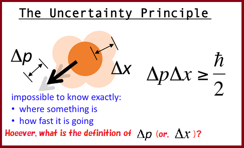
“Б‚ЙЃB‚а‚µ$A_1 A_2 - A_2 A_1 = \hbar \sqrt{-1}$
‚И‚з‚ОЃAЋџ‚Єђ¬—§‚·‚йЃF
\begin{align}
&
{\Delta}_{\widehat{N}_1}^{{\widehat{\rho}_{us}}} \cdot { \Delta}_{\widehat{N}_2}^{{\widehat{\rho}_{us}}}
\ge \hbar/2
\quad ( \forall u \in H \mbox{ such that } ||u||=1 )
\\
&
\tag{4.35}
\end{align}
|
‹ЯЋ—“ЇЋћ‘Є’и‚М‘¶ЌЭ’и—ќ(i)‚ЖѓnѓCѓ[ѓ“ѓxѓ‹ѓO‚М•sЉm’иђ«ЉЦЊW(ii)‚МЏШ–ѕ‚Н,Ћџ‚рЊ©‚ж.
ѓnѓCѓ[ѓ“ѓxѓ‹ѓO‚М•sЉm’иђ«Њґ—ќ(ii)‚МЏШ–ѕ‚Н,(4.32})‚ЕЋ¦‚µ‚Ѕ‚悤‚ЙЉИ’P‚Е‚ ‚й‚Є,‹ЯЋ—“ЇЋћ‘Є’и‚М‘¶ЌЭ’и—ќ(i)‚Н‘ЅЏ“п‚µ‚ў.
