哲学には、「だれも理解していないのに、世論を動かした仕事」が数多くあって(というより、哲学の大抵の仕事はそうだと思う)、本書でも逐次述べていく。
たとえば、ウィトゲンシュタインの
などで、こいう言葉に感心する人の気がしれないと思っていたが(多分、ホーキング博士も否定的だと思う(cf. $\S$19.3)、
しかも、ウィトゲンシュタインだって本当にわかって発言したかどうかは疑わしいが、
本書では、 量子言語からの視点から随所にこの言葉の重要性を強調すだろう。
EPR論文もあとあと結構使う。
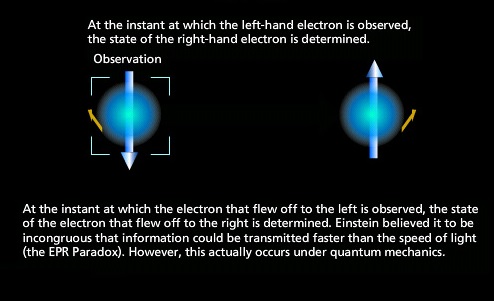
$\S$4.4.1: EPR-パラドックスと超光速
$2$個の電子$P_1$と
$P_2$の
スピン状態
を考える.
このために,
テンソルヒルベルト空間
$H={\mathbb C}^2 \otimes {\mathbb C}^2$
を次のように定める.
すなわち,
(i.e., 完全正規直交系 $\{ e_1, e_2 \}$ in ${\mathbb C}^2$),
ここで,
$u=\sum\limits_{i,j=1,2} \alpha_{ij} e_i \otimes e_j$
と
$v=\sum\limits_{i,j=1,2} \beta_{ij} e_i \otimes e_j$の内積
$\langle u,v \rangle_{_{{\mathbb C}^2 \otimes {\mathbb C}^2}}$
を
\begin{align*}
\langle u,v \rangle_{_{{\mathbb C}^2 \otimes {\mathbb C}^2}}
=
\sum\limits_{i,j=1,2} \overline{\alpha}_{i,j}\cdot \beta_{i,j}
\end{align*}
で定める.
したがって,
テンソルヒルベルト空間
$H={\mathbb C}^2 \otimes {\mathbb C}^2$
の
完全正規直交基底を
$\{ e_1 \otimes e_1,
e_1 \otimes e_2,
e_2 \otimes e_1,
e_2 \otimes e_2
\}$
と定めたことになる.
また,$F\in B({\mathbb C}^2)$,
$G\in B({\mathbb C}^2)$に対して,
$F\otimes G \in B({\mathbb C}^2 \otimes {\mathbb C}^2)$
(すなわち,
線形写像$F\otimes G : {\mathbb C}^2 \otimes {\mathbb C}^2
\to
{\mathbb C}^2 \otimes {\mathbb C}^2
$
)
を
によって定める.
2個の電子$P_1$と
$P_2$の
シングレット状態
(
双子状態,エンタングル状態,もつれ状態
とも言う)
$|s \rangle \langle s |
(\in
\in {\mathbb C}^2 \otimes {\mathbb C}^2
)
$
を次で定める.
ここに,
$\langle s,s \rangle_{_{{\mathbb C}^2 \otimes {\mathbb C}^2}}$
$=\frac{1}{2}\langle e_1\otimes e_2 - e_2 \otimes e_1 ,e_1\otimes e_2 - e_2 \otimes e_1 \rangle_{_{{\mathbb C}^2 \otimes {\mathbb C}^2}}$
$=\frac{1}{2}(1+1)=1$
により,
$|s \rangle \langle s |
$は状態
であることは明らか.
また,
しかし、これは非常に難解な(というより整理されていない)論文で、評価の難しい論文だと思う。 エンタングル状態の発見者は誰だか知らないが、 多分アインシュタインではないだろう。
そうならば、だれも理解していないのに、なんとなく世間が騒いで、
という論文だと思う。
否定的なことを言っているのではない。
「こういう形で影響力を持つ論文」もあるとのかと感心しているのである。
「何があるか?」の解答は、このページの下の「注釈4.4」に書くが、この視点(量子言語からの視点)無くして、EPRの意味が分かるはずはない思うからである。
$(\sharp_1):$
The limits of my language mean the limits of my world
(私の言語の限界が、私の世界の限界)
$(\sharp_2):$
What we cannot speak about we must pass over in silence
(語り得ぬことは、沈黙しなければならない)
と仮定してもよいことには
注意しておく.
さて,
シュテルン=ゲルラッハの実験のときと
同様に,
$B({\mathbb C}^2)$
内の$z$-方向のスピン観測量${\mathsf O} =(X,2^X, F^z )$
を,$X=\{\uparrow ,\downarrow \}$
として,
で定めて, $B({\mathbb C}^2\otimes {\mathbb C}^2)$ 内の並行観測量${\mathsf O}\otimes {\mathsf O} =(X^2,2^X\times 2^X, F^z \otimes F^z)$ を
\begin{align} & (F^z \otimes F^z)(\{(\uparrow,\uparrow )\})=F^z(\{\uparrow \}) \otimes F^z(\{\uparrow \}) = \left[\begin{array}{ll} 1 & 0 \\ 0 & 0 \end{array}\right] \otimes \left[\begin{array}{ll} 1 & 0 \\ 0 & 0 \end{array}\right] \;\; \\ & (F^z \otimes F^z)(\{(\downarrow,\uparrow )\})=F^z(\{\downarrow \}) \otimes F^z(\{\uparrow \}) = \left[\begin{array}{ll} 0 & 0 \\ 0 & 1 \end{array}\right] \otimes \left[\begin{array}{ll} 1 & 0 \\ 0 & 0 \end{array}\right] \\ & (F^z \otimes F^z)(\{(\uparrow,\downarrow )\})=F^z(\{\uparrow \}) \otimes F^z(\{\downarrow \}) = \left[\begin{array}{ll} 1 & 0 \\ 0 & 0 \end{array}\right] \otimes \left[\begin{array}{ll} 0 & 0 \\ 0 & 1 \end{array}\right] \;\;\\ & (F^z \otimes F^z)(\{(\downarrow,\downarrow )\})=F^z(\{\downarrow \}) \otimes F^z(\{\downarrow \}) = \left[\begin{array}{ll} 0 & 0 \\ 0 & 1 \end{array}\right] \otimes \left[\begin{array}{ll} 0 & 0 \\ 0 & 1 \end{array}\right] \end{align}によって定める. このようにして, 測定 ${\mathsf M}_{B({\mathbb C}^2\otimes {\mathbb C}^2)}({\mathsf O}\otimes {\mathsf O},S_{[ |s \rangle \langle s | ]})$ を得る. このとき,ボルンの量子測定理論 [(量子版)言語ルール1] によって,次が言える:
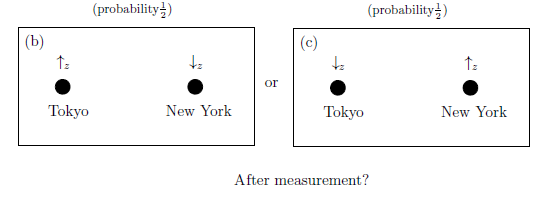
| $\quad$ | 測定 ${\mathsf M}_{B({\mathbb C}^2\otimes {\mathbb C}^2)}({\mathsf O}\otimes {\mathsf O},S_{[ |s \rangle \langle s | ]})$ により \begin{align} & \text{測定値} \left[\begin{array}{ll} (\uparrow,\uparrow ) \\ (\downarrow,\uparrow ) \\ (\uparrow,\downarrow ) \\ (\downarrow,\downarrow ) \end{array}\right] \text{を得る確率は} \left[\begin{array}{ll} \langle s, (F^z \otimes F^z)(\{(\uparrow,\uparrow )\})s \rangle_{_{{\mathbb C}^2 \otimes {\mathbb C}^2}} = 0 \\ \langle s, (F^z \otimes F^z)(\{(\downarrow,\uparrow )\})s \rangle_{_{{\mathbb C}^2 \otimes {\mathbb C}^2}} = 0.5 \\ \langle s, (F^z \otimes F^z)(\{(\uparrow,\downarrow )\})s \rangle_{_{{\mathbb C}^2 \otimes {\mathbb C}^2}} = 0.5 \\ \langle s, (F^z \otimes F^z)(\{(\downarrow,\downarrow )\})s \rangle_{_{{\mathbb C}^2 \otimes {\mathbb C}^2}} = 0 \end{array}\right] \\ & \tag{4.46} \end{align} である。 |
なぜならば, $F^z (\{\uparrow \})e_1=e_1$, $F^z (\{\downarrow \})e_2=e_2,F^z (\{\uparrow \})e_2= F^z (\{\downarrow \})e_1=0$であり、 たとえば,
\begin{align} & \langle s, (F^z \otimes F^z)(\{(\uparrow,\downarrow )\})s \rangle_{_{{\mathbb C}^2 \otimes {\mathbb C}^2}} \\ = & \frac{1}{2}\langle (e_1\otimes e_2 - e_2 \otimes e_1 ) , (F^z(\{\uparrow \}) \otimes F^z(\{\downarrow \}) (e_1\otimes e_2 - e_2 \otimes e_1 ) \rangle_{_{{\mathbb C}^2 \otimes {\mathbb C}^2}} \\ = & \frac{1}{2}\langle (e_1\otimes e_2 - e_2 \otimes e_1 ) , e_1\otimes e_2 \rangle_{_{{\mathbb C}^2 \otimes {\mathbb C}^2}} = \frac{1}{2} \end{align} だからである。ここで、 測定値$x_1$と$x_2$ (in $(x_1, x_2)$ $ \in $ $\{$ $ (\uparrow _{z},\uparrow _{z}),$ $ (\uparrow _{z},\downarrow _{z}),$ $ (\downarrow _{z},\uparrow _{z}), (\downarrow _{z},\downarrow _{z}) \}$)がそれぞれ東京とニューヨーク(もっと極端には、地球と北極星)で得られたと仮定しよう。
上の議論は, $A_1$地点(地球上)で粒子$P_1$に対する 測定値「$\downarrow$」 を得たとすれば, 何光年も遠く離れた $A_2$地点(北極星)の粒子$P_2$に対しては 測定値「$\uparrow$」 が得られることを意味する. これは不可思議である.
この不思議さを説明するには、次しかない。
| $\bullet$ | $A_1$地点で,粒子$P_1$が 測定値「$\downarrow$」を測定された 瞬間に,粒子$P_1$ が,その事実を$A_2$地点の粒子$P_2$に 超光速で伝達して, 『私は「$\downarrow$」と測定されたから, 君は「$\uparrow$」と測定されるようにしなさい』 と 伝えた |
と考えたくなる. このような シングレット状態に関する議論を, 総称して,EPR-パラドックスと呼ぶ.
「超光速(=非局所性)」という意味では、EPR-パラドックスもド・ブロイのパラドックスも同じである。 と言うより,
| $\bullet$ | 言語ルール1(=ボルンの量子測定)を使うときには、いつも必ず「超光速(=非局所性)」のパラドックスが現れる。 |
| $\fbox{注釈4.4}$ |
EPR-パラドックスはいろいろな側面がある。
第8章では、
「三段論法の非成立」について述べる。
EPR-パラドックスに関しての
「ボーア=アインシュタイン論争」
は、
20世紀最大の科学論争であるが、本書の「量子言語の立場」では、次のように理解したい:
\begin{align*}
\underset{\mbox{(実在的科学観)}}{\fbox{$\mbox{アインシュタイン}$}}
\quad
\underset{\mbox{v.s.}}{\longleftrightarrow}
\quad
\underset{\mbox{ (言語的科学観)}}{\fbox{$\mbox{ボーア}$}}
\end{align*}
もちろん、ボーア等は、彼らが作り上げたコペンハーゲン解釈を物理学と信じていたに違いない。
しかし、作品が作家の意図とは別の意味をもつことはよくあることと思う。
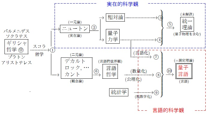
「実在的科学観 vs. 言語的科学観」は、
「アリストテレス vs. プラトン」以来いろいろな形で現れる科学における最大の論争である。
と言うより、
この議論は $\S$10.7 (ライプニッツ=クラーク論争) で再考する。 本書の目的は、「実在的科学観(唯物論) vs. 言語的科学観(観念論)」を、お互いの顔が立つように収めることであるとも言える (右の図1.1 in $\S$1.1 参照). |
