以下に,実現因果観測量に関する定理・定義を述べる.
この節では,「有限実現因果観測量」に限定するので,いずれも容易に理解できると思う.理論的観点からは,
次節の「無限実現因果観測量」のための準備であるが,
応用的には,「有限実現因果観測量」でも十分使える.
を考える.
$\Phi_{1,2}:\overline{\mathcal A}_2
\to
\overline{\mathcal A}_1$を因果作用素とする.
このとき,
${\overline{\mathcal A}_2}$内の任意の観測量
$
{\mathsf O}_2$
$=$
$(X , {\cal F} , F_2{})$
に対して,
$(X , {\cal F} , \Phi_{1,2} F_2{})$
は${\overline{\mathcal A}_1}$内の観測量
である.これを$\Phi_{1,2} {\mathsf O}_2$
$=$
$(X , {\cal F} , \Phi_{1,2} F_2{})$
と記す.
この節では,木半順序集合$T(t_0)$
が有限の場合を考える.
$T(t_0)
= \{ t_0, t_1,\ldots , t_N \}$
として,
ルート$t_0$
をもつ木半順序集合
$(T(t_0), {{\; \leqq \;}})$
を考える.
その親写像表現を
$(T{{=}} \{ t_0,t_1,\ldots, t_N\} , \pi:
T \setminus \{ t_0 \} \to T)$
とする.
として,因果作用素列
$\{ \Phi_{t_1,t_2}{}: $
$\overline{\mathcal A}_{t_2}
\to
\overline{\mathcal A}_{t_1}
\}_{(t_1,t_2) \in T^2_{\leqq}}$
を考える.すなわち, 次を満たすとする(
cf.
定義10.10
):
各
$t \in T$に対して,
$\overline{\mathcal A}_{t}
$内の観測量${\mathsf O }_t {{=}} (X_t, {\cal F}_t , F_t{})$
を
定める.
対
$[{}\{ {\mathsf O}_t \}_{ t \in T} ,
\{ \Phi_{t_1,t_2}{}: $
$\overline{\mathcal A}_{t_2}
\to
\overline{\mathcal A}_{t_1}
\}_{(t_1,t_2) \in T^2_{\leqq}}$
$]$
を
因果観測量列
と呼び,
$[{}{\mathsf O}_T{}]$
または
$[{}{\mathsf O}_{T(t_0)}{}]$
と記す.
すなわち,
$[{}{\mathsf O}_T{}]$
$=$
$[{}\{ {\mathsf O}_t \}_{ t \in T} ,
\{ \Phi_{t_1,t_2}{}: $
$
\overline{\mathcal A}_{t_2}
\to
\overline{\mathcal A}_{t_1}
\}_{(t_1,t_2) \in T^2_{\leqq}}$
$]$
である.
木半順序集合$T(t_0)
= \{ t_0, t_1,\ldots , t_N \}$が有限のとき,
親写像$\pi: T\setminus \{t_0\} \to T$
を使って,
$[{}{\mathsf O}_T{}]$
$=$
$[{}\{ {\mathsf O}_t \}_{ t \in T} ,
$
$
\{
\overline{\mathcal A}_{t}
\xrightarrow[]{{\Phi_{ \pi(t{}), t } }}
\overline{\mathcal A}_{\pi(t)}
\}_{t \in T \setminus \{ t_0 \}{}) {}}]$
と書くこともある.
問題12.3
この問題を解くためには,言語的解釈(=言語的コペンハーゲン解釈)に頼らなければならない.
言語的解釈
─
測定理論の解釈
─
では,
「測定は一回だけ」
で,
したがって,
「観測量は一つだけ」
が要請される.
このために,
因果観測量列
$[{}{\mathsf O}_T{}]$
${{=}}$
$[{}\{ {\mathsf O}_t \}_{ t \in T} ,
\{ \Phi_{t_1,t_2}{}: $
$\overline{\mathcal A}_{t_2}
\to
\overline{\mathcal A}_{t_1}
\}_{(t_1,t_2) \in T^2_{\leqq}}$
$]$
の中の多数の観測量
${}\{ {\mathsf O}_t \}_{ t \in T} $
を
一つに合体させなければならい.
これは,次の実現因果観測量によって
実現される.
$[{\mathsf O}_{T(t_0)}]$
$=$
$[{}\{ {\mathsf O}_t \}_{ t \in T},
\{ \Phi_{\pi(t), t }{}: $
$\overline{\mathcal A}_{t} $
$
\xrightarrow[]{{\Phi_{ \pi(t{}), t } }}
$
$
\overline{\mathcal A}_{\pi(t)}
\}_{ t \in T\setminus \{t_0\} }$
$]$
を
因果観測量列
とする.
各 $s$
$(\in T{})$に対して,
$T_s = \{ t \in T \;|\; t {\; \geqq \;}s \}$
とおく.
$
\overline{\mathcal A}_{s}
$内の
{{}}観測量
$\widehat{\mathsf O}_s {{=}} ({{{\times}}}_{t \in T_s } X_t, $
$\boxtimes_{t \in T_s } {\cal F}_t, {\widehat F}_s)$
を以下の規則で定める:
$\;\;$
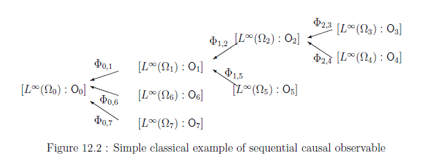
$\pi(1) = \pi(6) = \pi(7) = 0$,
$\pi(2) = \pi(5) = 1$,
$\pi(3) = \pi(4) = 2$.
さて,
因果観測量列
$[{}{\mathsf O}_T{}]$
$=$
$[{}\{ {\mathsf O}_t \}_{ t \in T} ,
$
$
\{
\overline{\mathcal A}_t
{{\Phi_{ \pi(t{}), t } }\atop{\rightarrow}} $
$
\overline{\mathcal A}_{\pi(t)}
\}_{t \in T \setminus \{ 0 \}{}) {}}]$
の
実現因果観測量$\widehat{\mathsf O}_{T(t_0){}}$
$=$
$({{{\times}}}_{t \in T } X_t, $
$\boxtimes_{t \in T } {\cal F}_t,$
${\widehat F}_{t_0})$を以下のように構成しよう.
$T \setminus \pi(T) =\{3,4,5,6,7\}$
であるから,
\begin{align*}
\widehat{\mathsf O}_t
=
{\mathsf O}_t,
\quad
\text{}
\quad
\widehat{F}_t
=
{F}_t
\quad
(t = 3,4,5,6,7)
\end{align*}
となる.
次に,$
\overline{\mathcal A}_2
$内の同時観測量
$
\widehat{\mathsf O}_2
= (X_2 \times X_3 \times X_4,
{\cal F}_2 \boxtimes {\cal F}_3 \boxtimes {\cal F}_4,
{\widehat F}_2 {})
$
を次のように構成する.
\begin{align*}
{\widehat F}_2
&
=
F_2 \times ({{{\times}}}_{t \in \pi^{-1}(\{2\})} \Phi_{\pi(t),t}
{\widehat F}_t{})
=
F_2 \times ({{{\times}}}_{t=3,4} \Phi_{2,t} {\widehat F}_t{})
=
F_2 \times ({{{\times}}}_{t=3,4} \Phi_{2,t} {F}_t{})
\\
&
=
F_2 \times \Phi_{2,3} {F}_3{}
\times
\Phi_{2,4} {F}_4{}
\end{align*}
(量子系の場合は,$\widehat{\mathsf O}_2$の存在は,保証されているわけでないことに注意せよ).
となって,
(12.3)式とは違う結果になってしまうので注意を要する.
以下の定理や例の中では,
存在観測量を省略して議論することもあるが,
その場合は細心の注意のもとに
省略していると思ってもらいたい.
二元論的言語(量子言語=測定理論)
では,
言語ルール2(因果関係)が単独で使われることはなくて,
常に言語ルール1(測定)と組みになっている.
なぜならば,同じ意味で,
$(A_1):$
測定してみなければ,なにもわからない
だからである。
$(A_2):$
存在するとは,知覚されること (by George Berkeley(1685年 - 1753年))

$\fbox{注釈12.1}$
バークリーの言葉
は、
アインシュタイン=タゴール会談での
アインシュタインの言葉:
$(\sharp_1):$
存在するとは、知覚されること
との対比
\begin{align*}
\underset{(運動方程式だけではダメで、測定が必須)}{
\fbox{$\qquad (\sharp_1):$二元論的観念論 $\qquad \qquad \qquad$}
}
\quad
\mbox{
vs.
}
\underset{(運動方程式だけでOK)}
{\fbox{
$(\sharp_2)$:一元論的実在論$\qquad \qquad $
}
}
\end{align*}
において、深淵である。
$(\sharp_2):$
月は、見ていても、見ていなくても存在する
(=[測定者がいなくても、物理学は成立する]
)
定理 12.1 [=定理 11.1:[因果作用素と観測量]]
一般の基本構造
\begin{align*}
[ {\mathcal A}_k \subseteq \overline{\mathcal A}_k \subseteq {B(H_k)}]
\qquad
(k=1,2)
\end{align*}
Proof
See proof of 定理 11.1.
定義12.2 [有限因果観測量列]
$\;$
一般の基本構造を
\begin{align*}
[ {\mathcal A}_k \subseteq \overline{\mathcal A}_k \subseteq {B(H_k)}]
\qquad
(t \in T(t_0)=\{t_0, t_1, \cdots, t_n \})
\end{align*}
$(i):$
任意の$(t_1,t_2) \in T^2_{\leqq}$に対して, 因果作用素
$\Phi_{t_1,t_2}{}: $
${
\overline{\mathcal A}_{t_2}} \to {\overline{\mathcal A}_{t_1}}$
が定義されて,
$\Phi_{t_1,t_2} \Phi_{t_2,t_3} = \Phi_{t_1,t_3}$
$(\forall (t_1,t_2)$,
$\forall (t_2,t_3) \in T^2_{\leqq})$
を満たす.
ここに,
$\Phi_{t,t} : {\overline{\mathcal A}_{t}} \to {\overline{\mathcal A}_{t}}$
は恒等作用素とする.

ここで、次の問題を考える。
初期純粋状態$\rho_{t_0}
\in {\frak S}^p({\mathcal A}_{t_0}^*)
$
を持つシステムに対しての
因果観測量列$[{}{\mathsf O}_T{}]$
$=$
$[{}\{ {\mathsf O}_t \}_{ t \in T} ,
\{ \Phi_{t_1,t_2}{}: $
$
\overline{\mathcal A}_{t_2}
\to
\overline{\mathcal A}_{t_1}
\}_{(t_1,t_2) \in T^2_{\leqq}}$
$]$の測定を,如何に定式化するか?
\begin{align}
\widehat{\mathsf O}_s
=
\begin{cases}
{\mathsf O}_s
\quad
&
\text{$ ( s \in T \setminus \pi (T) \; \text{のとき}${})}
\\
\\
{\mathsf O}_s
{\times}
({{{\times}}}_{t \in \pi^{-1} (\{ s \}{})} \Phi_{ \pi(t), t} \widehat {\mathsf O}_t{})
\quad
&
\text{($ s \in \pi (T) \; \text{のとき}${})}
\end{cases}
\tag{12.1}
\end{align}
(量子系の場合は,$\widehat{\mathsf O}_s$の存在は,保証されているわけでないことに注意せよ).
これを逐次的に用いて,
結局,
$
\overline{\mathcal A}_{t_0}
$
内の観測量
$\widehat{\mathsf O}_{t_0{}}$
$=$
$({{{\times}}}_{t \in T } X_t, $
$\boxtimes_{t \in T } {\cal F}_t,$
${\widehat F}_{t_0})$
を得る.
$\widehat{\mathsf O}_{t_0{}}$
$=$
$\widehat{\mathsf O}_{T(t_0){}}$
とおく.
$\widehat{\mathsf O}_{T(t_0){}}$
$=$
$({{{\times}}}_{t \in T } X_t, $
$\boxtimes_{t \in T } {\cal F}_t,$
${\widehat F}_{t_0})$
を,
(有限)因果観測量列$[{}{\mathsf O}_{T(t_0)}{}]$
$=$
$[{}\{ {\mathsf O}_t \}_{ t \in T} ,
\{ \Phi_{\pi(t), t }{}: $
$\overline{\mathcal A}_{t}
\to
\overline{\mathcal A}_{\pi(t)}
\}_{ t \in T\setminus \{t_0\} }$
$]$
の
(有限)実現因果観測量
と呼ぶ.
$\fbox{注釈12.2}$
上の
(12.1)
式において、
積"$\times$"を擬積"$\mathop{\times}^{qp}$"に置き換えてもよいが、
本書では、これに関わらない。
例 12.5 [単純な例(図11.3
から続く)]
更に,
$
\overline{\mathcal A}_1$内の同時観測量
$
\widehat{\mathsf O}_1
=
$
$(X_1 \times X_2 \times X_3 \times X_4
\times X_5, {\cal F}_1 \boxtimes {\cal F}_2 \boxtimes {\cal F}_3 \boxtimes {\cal F}_4
\boxtimes {\cal F}_5,
{\widehat F}_1 {})
$
を次のように構成する.
\begin{align*}
{\widehat F}_1
=
F_1 \times ({{{\times}}}_{t=2,5} \Phi_{1,t} {\widehat F}_t{})
=
F_1
\times
\Phi_{1,5}F_5
\times
\Phi_{1,2}
\Big(
F_2
\times \Phi_{2,3}F_3
\times \Phi_{2,4}F_4
\Big)
\end{align*}
そして,
結局,
$\overline{\mathcal A}_0$内の
実現因果観測量
$
\widehat{\mathsf O}_0
=
$
$({{{\times}}}_{t=1}^7 X_t , \boxtimes_{t=1}^7 {\cal F}_t,
{\widehat F}_0 {})
$
を以下のように構成できる.
\begin{align*}
{\widehat F}_0
=
F_0 \times ({{{\times}}}_{t=1,6,7} \Phi_{0,t} {\widehat F}_t{})
\end{align*}
上の手続きを図示すると
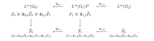
このようにして,
因果観測量列
$[{}\{{\mathsf O}_t\}_{t \in T },$
$\{ \overline{\mathcal A}_t \overset{\Phi_{\pi(t), t}}\to$
$\overline{\mathcal A}_{\pi(t)} \}_{ t \in T \setminus \{0\} }{}]$
の
実現因果観測量$\widehat{\mathsf O}_{0{}}$
$=$
$\widehat{\mathsf O}_{T{}}$
を得る.
${\widehat F}_0
$
を書き下すと,
\begin{align}
&
\widehat{F}_0 (\Xi_0 \times \Xi_1 \times \Xi_2 \times \Xi_3 \times \Xi_4 \times \Xi_5 \times \Xi_6 \times \Xi_7)]
\nonumber
\\
=
&
F_0(\Xi_0)
\times
\Phi_{0,1} \biggl(
F_1(\Xi_1)
\times
\Phi_{1,5}F_5(\Xi_5)
\times
\Phi_{1,2}
\Big(
F_2(\Xi_2) \times \Phi_{2,3}F_3(\Xi_3)
\times \Phi_{2,4}F_4(\Xi_4)
\Big)
\biggl)
\nonumber
\\
&
\qquad
\qquad
\times
\Phi_{0,6}(
F_6(\Xi_6))
\times
\Phi_{0,7}(
F_7(\Xi_7))
\tag{12.2}
\end{align}
となる.(量子系の場合は,$\widehat{\mathsf O}_0$の存在は,保証されているわけでないことに注意せよ).
注意12.6
上で,$t=2,6,7$
で,
${\mathsf O}_t$
が定まっていないとしたら,
$t=2,6,7$
に対して,
存在観測量
${\mathsf O}^{\text{存}}_t {{=}} (X_t ,
\{ \emptyset, X_t \}, F^{\text{存}}_t)$
(cf.例2.20)
を想定すればよい.
そうすれば,
$[
F^{\text{存}}_t
(X_t)](\omega)=1$
$(t=2,6,7)$
だから,
\begin{align}
&
\widehat{F}_0 (\Xi_0 \times \Xi_1 \times
X_2 \times \Xi_3 \times \Xi_4 \times \Xi_5 \times X_6
\times X_7
)
\nonumber
\\
=&
F_0(\Xi_0)
\times
\Phi_{0,1} \biggl(
F_1(\Xi_1)
\times
\Phi_{1,5}F_5(\Xi_5)
\times
\Phi_{1,2}
\Big(
\Phi_{2,3}F_3(\Xi_3)
\times \Phi_{2,4}F_4(\Xi_4)
\Big)
\biggl)
\tag{12.3}
\end{align}
となる.
存在観測量を考えないで,
$T'$
$=$
$\{0,1,3,4,5 \}$
として,
$[{}{\mathsf O}_{T'}{}]$
$=$
$[{}\{ {\mathsf O}_t \}_{ t \in {T'}} ,$
$
\{ \Phi_{t_1,t_2}{}: $
${\overline{\mathcal A}_{t_2}} \to {\overline{\mathcal A}_{t_1}} \}_{(t_1,t_2) \in (T')^2_{{\; \leqq \;}}}$
$]$
とすると,その実現因果観測量
$\widehat{\mathsf O}_{T'(0){}}$
$=$
$({{{\times}}}_{t \in T' } X_t, $
$\boxtimes_{t \in T' } {\cal F}_t,$
${\widehat F}'_{0})$
は,
\begin{align}
&
\widehat{F}'_0 (\Xi_0 \times \Xi_1 \times
\Xi_3 \times \Xi_4 \times \Xi_5
)
\nonumber
\\
=
&
F_0(\Xi_0)
\times
\Phi_{0,1} \Big(
F_1(\Xi_1)
\times
\Phi_{1,5}F_5(\Xi_5)
\times
\Phi_{1,4}F_4(\Xi_4)\times \Phi_{1,3}F_3(\Xi_3)
\times \Phi_{1,4}F_4(\Xi_4)
\Big)
\tag{12.4)}
\end{align}
以上により,問題12.3に次のように答えることができる.
問題12.7 [=問題12.3の再掲]
初期状態$\rho_{t_0}
\left\{\begin{array}{lll}
\in {\frak S}^p({\mathcal A}_{t_0}^*):\;\; \mbox{純粋状態}
\\
\in \overline{\frak S}^m((\overline{\mathcal A}_{t_0})_*):\;\; \mbox{$W^*-$混合状態}\quad
\\
\in {\frak S}^m({\mathcal A}_{t_0}^*):\;\; \mbox{$C^*-$混合状態}
\end{array}\right\}
$
を持つシステムに対しての
因果観測量列$[{}{\mathsf O}_T{}]$
$=$
$[{}\{ {\mathsf O}_t \}_{ t \in T} ,
\{ \Phi_{t_1,t_2}{}: $
$
\overline{\mathcal A}_{t_2}
\to
\overline{\mathcal A}_{t_1}
\}_{(t_1,t_2) \in T^2_{\leqq}}$
$]$の測定を,如何に定式化するか?
解答
実現観測量$\widehat{\mathsf O}_{t_0}$が存在するならば,
\begin{align*}
\left\{\begin{array}{lll}
\mbox{
純粋測定}
{\mathsf M}_{\overline{\mathcal A}_{t_0}}(\widehat{\mathsf O}_{t_0}, S_{[\rho_{t_0}]})
\\
\mbox{
$W^*-$混合測定}
{\mathsf M}_{\overline{\mathcal A}_{t_0}}(\widehat{\mathsf O}_{t_0}, S_{[\ast]}{(\rho_{t_0})}) \quad
\\
\mbox{
$C^*-$混合測定}
{\mathsf M}_{\overline{\mathcal A}_{t_0}}(\widehat{\mathsf O}_{t_0}, S_{[\ast]}{(\rho_{t_0})})
\end{array}\right\}
\end{align*}
と定式化できる.
実現因果観測量
$\widehat{\mathsf O}_{T{}}
(=
\widehat{\mathsf O}_{t_0{}}
)$
に,
言語ルール1(純粋測定)を適用すれば,
| $(B_1):$ | 測定 ${\mathsf M}_{\overline{\mathcal A}_{t_0}}(\widehat{\mathsf O}_{T{}}, S_{[\rho_{t_0}]})$ により得られる測定値 $(x_t)_{t \in T}$ が ${\widehat \Xi}( \in \boxtimes_{t\in T}{\cal F}_t )$ に属する確率は, \begin{align} {}_{{\mathcal A}^*} \Big( \rho_{t_0}, {\widehat F}_{t_0} ({\widehat \Xi} ) \Big) {}_{\overline{\mathcal A}_{t_0}} \tag{12.5} \end{align} となる. |
いずれにしても、
| $(B_2):$ | 初期状態$\rho_0$は固定されていて, 状態は変化しない. |
定理 12.8[決定的因果観測量列の実現因果観測量 ]
有限木半順序集合を
$(T(t_0), {{\; \leqq \;}})$
とする.
各$t \in T(t_0)$に対して,古典系の基本構造
\begin{align*}
[C_0(\Omega_t) \subseteq L^\infty (\Omega_t, \nu_t ) \subseteq
B(L^2 (\Omega_t, \nu_t ))]
\end{align*}
を考える.
因果観測量列$[{}{\mathsf O}_T{}]$
$=$
$[{}\{ {\mathsf O}_t \}_{ t \in T} ,
\{ \Phi_{t_1,t_2}{}: $
${L^\infty (\Omega_{t_2})} \to {L^\infty (\Omega_{t_1})} \}_{(t_1,t_2) \in T^2_{\leqq}}$
$]$
において,
$\{ \Phi_{t_1,t_2}{}: $
${L^\infty (\Omega_{t_2})} \to {L^\infty (\Omega_{t_1})} \}_{(t_1,t_2) \in T^2_{\leqq}}$
が決定的因果作用素列ならば,
実現因果観測量$\widehat{\mathsf O}_{T({t_0}){}} $
は
次のように表現できる:
\begin{align*}
\widehat{\mathsf O}_{T({t_0}){}} = {{{\times}}}_{t\in T} \Phi_{{t_0},t} {\mathsf O}_t
\end{align*}
すなわち,
\begin{align*}
&
[\widehat{F}_{t_0} (
{{{\times}}}_{t\in T} \Xi_t \
)]
(\omega_{t_0} ) = {{{\times}}}_{t\in T} [\Phi_{{t_0},t} {F}_t (\Xi_t )](\omega_{t_0} )
= {{{\times}}}_{t\in T} [{F}_t (\Xi_t )](\phi_{{t_0},t} \omega_{t_0} )
\\
&
\quad \qquad \quad \qquad \quad \qquad \quad \qquad
(\forall \omega_{t_0} \in \Omega_{t_0}, \forall \Xi_t \in {\cal F}_t )
\end{align*}
が成立する.
証明
一般の場合も同様なので,
例12.5(すなわち,図13.1)の場合について示す.
定理10.6定理を繰り返し使って,
\begin{align*}
&
{\widehat F}_0
=
F_0 \times ({{{\times}}}_{t=1,6,7} \Phi_{0,t} {\widehat F}_t{})
\\ %一行目
=
&
F_0 \times (
\Phi_{0,1} {\widehat F}_1{}
\times
\Phi_{0,6} {\widehat F}_6{}
\times
\Phi_{0,7} {\widehat F}_7{}
)
=
F_0 \times (
\Phi_{0,1} {\widehat F}_1{}
\times
\Phi_{0,6} {F}_6{}
\times
\Phi_{0,7} { F}_7{}
)
\\ %二行目
=
&
\Big(
{{{\times}}}_{t=0,6,7}
\Phi_{0,t} F_t
\Big)
\times (
\Phi_{0,1} {\widehat F}_1{}
)
=
\Big({{{\times}}}_{t=0,6,7}
\Phi_{0,t} F_t
\Big)
\times
\Phi_{0,1}
(
F_1 \times ({{{\times}}}_{t=2,5} \Phi_{1,t} {\widehat F}_t{})
{}
)
\\
=
&
\Big(
{{{\times}}}_{t=0,1,6,7}\Phi_{0,t} F_t
\Big)
\times
\Phi_{0,1}({{{\times}}}_{t=2,5} \Phi_{1,t} {\widehat F}_t{})
\\
=
&
\Big(
{{{\times}}}_{t=0,1,6,7}\Phi_{0,t} F_t
\Big)
\times
\Phi_{0,1}(
\Phi_{1,2} {\widehat F}_2{}
\times
\Phi_{1,5} {\widehat F}_5{})
\\ %三行目
=
&
\Big(
{{{\times}}}_{t=0,1,5,6,7}\Phi_{0,t} F_t
\Big)
\times
\Phi_{0,1}(
\Phi_{1,2} {\widehat F}_2{}
)
\\
=
&
\Big(
{{{\times}}}_{t=0,1,5,6,7}\Phi_{0,t} F_t
\Big)
\times
\Phi_{0,1}(
\Phi_{1,2}
(F_2 \times ({{{\times}}}_{t=3,4} \Phi_{2,t} {\widehat F}_t{}))
{}
)
\\
=
&
{{{\times}}}_{t=0}^7 \Phi_{0,t} F_t
\end{align*}
を得る.
