12.3: 二重スリット問題におけるウィルソンの霧箱
この節では、
ウィルソンの霧箱
(
i.e.,容器内の過飽和蒸気を荷電粒子が通過すると霧滴が生じて飛行機雲のように荷電粒子の軌跡がわかる現象を観測 するもの)
の一つのモデルを議論する。
(cf.
文献
\cite[(1991, 1994, S. Ishikawa, {\it et al.})]{IINT1, IINT2}
).
12.3.1: 量子粒子の厳密な軌道は無意味だが、近似的ならば、...
一次元実空間${\mathbb R}$
内の
粒子$P$の初期状態を
$| u \rangle \langle u |$とする。
ここに、
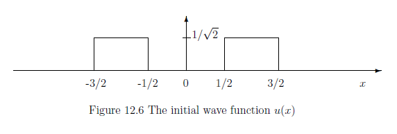
波動関数$u(x) \in H=L^2({\mathbb R})$.
を
次のように仮定する:
\begin{align}
u(x)
=
\begin{cases}
l/{\sqrt 2} , x\in ( -3/2, - 1/2) \cup (1/2, 3/2)
\\
\\
0, \mbox{ otherwise }
\end{cases}
\tag{12.8}
\end{align}
$A_0$を$B(H)$内の位置観測量(の自己共役作用素表現)とする。
すなわち、
\begin{align*}
(A_0v)(x)=xv(x)
\qquad
(\forall x \in {\mathbb R},
\qquad
(
\forall
v \in H=L^2({\mathbb R})
\end{align*}
この観測量表現は、$A_0$のスペクトル分解
${\mathsf O}=({\mathbb R}, {\mathcal B}_{{\mathbb R}},
E_{A_0})$
で表現される.
すなわち、
\begin{align*}
A_0 = \int_{\mathbb R} x E_{A_0} (d x )
\end{align*}
さて、次のハイゼンベルグの方程式を考える:
\begin{align}
- i \hbar \frac{dA_t}{dt}
={\mathcal H} A_t - A_t {\mathcal H},
\quad
-\infty
< t < \infty, \mbox{ where } A_0=A
\tag{12.9}
\end{align}
ここで、
ハミルトニアンは
$
{\mathcal H} = -(\hbar^2/2m)\partial^2 /\partial x^2
$
(すなわち、
ポテンシャル$V(x)=0$)
と仮定する。
ここで、
$U_t=$
$\exp(-itA)$
とおいて、
次を得る。
\begin{align}
A_t = U_t^* AU_t = U^*_txU_t = x +\frac{\hbar t}{im} {\frac{d}{dx}}
\tag{12.10}
\end{align}
ここで、$t=1/4$,
$\hbar/m=1$
とおいて、
さらに、
\begin{align*}
A=A_0(=x), \qquad B=A_{1/4}(=x+ \frac{1 }{4i} {\frac{d}{dx}})
=U_{1/4}^* A_0U_{1/4}=\Phi_{0, 1/4}A_0
\end{align*}
として、次の因果作用素を得る:
\begin{align*}
\underset{\mbox{初期波動関数:$u_0$}}{
\overset{\mbox{位置観測量: $A_0$}}{\fbox{$B(H_0)$}}}
\xleftarrow[\mbox{$\quad \Phi_{0,1/4} \quad $}]{}
\overset{\mbox{位置観測量: $A_0$}}{\fbox{$B(H_{1/4})$}}
\end{align*}
しかしながら、, $A_0(=A)$
と$\Phi_{0,1/4} A_0(=B)$
は非可換で、すなわち、
\begin{align*}
AB-BA=
x (x+ \frac{1 }{4i} {\frac{d}{dx}})-(x+ \frac{1 }{4i} {\frac{d}{dx}})x=i/4
\not=0
\end{align*}
となる。
したがって、
実現因果観測量は存在しない.
この意味では、
12.3.2: そうならば、近似的軌道を考える
粒子$P$の軌道は厳密な意味では無意味であるが、
近似的には意味を持つ。
これを以下のように考える。
自己共役作用素の組$\{A,B \}$
の近似同時測定(=
定義4.13
)
を復習しよう。
定義12.12(=定義4.13)
$A$と$B$をヒルベルト空間$H$上の自己共役作用素とする。
4つ組$(K, s, \widehat{A}, \widehat{B})$
が次を満たすとき、
$A$と$B$の
近似同時観測量
と呼ぶ。
| $(A_1):$ |
$K$はヒルベルト空間、.
$s \in K$,
$\| s \|_K=1$とする。
$\widehat{A}$と$\widehat{B}$
はテンソルヒルベルト空間$H \otimes K$
上の可換な自己共役作用素で、次の平均値一致条件を満たす:
\begin{align}
&
\langle u \otimes s, {\widehat A}(u \otimes s) \rangle
=
\langle u , {A} u \rangle,
\qquad
\langle u \otimes s, {\widehat B}(u \otimes s) \rangle
=
\langle u , {B} u \rangle
\tag{12.11}
\\
&
\qquad
\qquad ( \forall u \in H,
\|u\|_H=1)
\nonumber
\end{align}
|
また,測定
${\mathsf{M}}_{B(H\otimes K)} ({\mathsf{O}_{{\widehat A}}}\times{\mathsf{O}_{{\widehat B}}},S_{[{\widehat \rho}_{us}]})$
は、${\mathsf{M}}_{B(H)} ({\mathsf{O}_{A}},$
$ S_{[\rho_u]})$
と
${\mathsf{M}}_{B(H)} ({\mathsf{O}_{B}},$
$ S_{[\rho_u]})$
との
近似同時測定
と呼ばれる。
ここに、
\begin{align*}
{\widehat \rho}_{us}= | u \otimes s \rangle \langle u \otimes s |
\qquad
( \|s \}_K=1)
\end{align*}
さらに、近似同時測定${\mathsf{M}}_{B(H\otimes K)} ({\mathsf{O}_{{\widehat A}}}\times{\mathsf{O}_{{\widehat B}}},S_{[{\widehat \rho}_{us}]})$の
誤差
を以下のように定義する:
| $(A_2):$ |
${\Delta}_{\widehat{N}_1}^{{\widehat{\rho}_{us}}}$
$(=
\|
(\widehat{A}-A \otimes I)(u \otimes s)
\|
)$,
$\qquad$
${ \Delta}_{\widehat{N}_2}^{{\widehat{\rho}_{us}}}$
$(=
\|
(\widehat{B}-B \otimes I)(u \otimes s)
\|
)$
|
さて、近似同時観測量
$(K, s, \widehat{A}, \widehat{B})$
を以下のように構成しよう。
\begin{align*}
K=L^2 ({\mathbb R}_y ),
\qquad
s(y) =
=
\Big(
\frac{\omega_1}{\pi}
\Big)^{1/4}
\exp
\Big(-
\frac{\omega_1 |y|^2}{2}
\Big)
\end{align*}
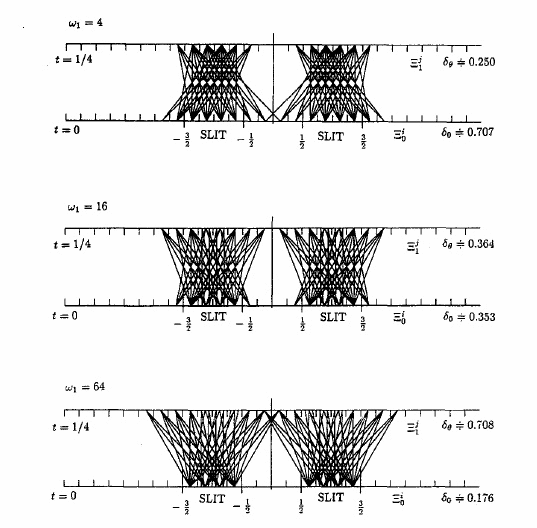
ここで$\omega_1$
は後に、$\omega_1=4,\;16,\;64$と考える.
ここで、
$\| s \|_{L^2({\mathbb R}_y)}=1$
(i.e.,
$\| s \|_K=1 $
)
として、次を満たすとしよう:
\begin{align}
\langle s, A s \rangle =\langle s, B s \rangle =0
\tag{12.12}
\end{align}
さらに、
\begin{align*}
&
{\widehat A}= A \otimes I + 2 I \otimes A
\\
&
{\widehat B}= B \otimes I - \frac{1}{2} I \otimes B
\end{align*}
として、
可換性
(i.e.,
$
{\widehat A}{\widehat B}
=
{\widehat B}{\widehat A}
$
)に注意しよう。
また、
(12.12)によって、
\begin{align}
&
\langle u \otimes s, {\widehat A}(u \otimes s) \rangle
=
\langle u \otimes s, ( { A}\otimes I +2 I \otimes A) (u \otimes s) \rangle
=
\langle u , {A} u \rangle
\tag{12.13}
\\
&
\langle u \otimes s, {\widehat A}(u \otimes s) \rangle
=
\langle u \otimes s, ( { B}\otimes I -2 I \otimes A) (u \otimes s) \rangle
=
\langle u , {B} u \rangle
\tag{12.14}
\\
&
\qquad ( \forall u \in H, i=1,2)
\nonumber
\end{align}
だから、
近似同時測定
${\mathsf{M}}_{B(H\otimes K)} ({\mathsf{O}_{{\widehat A}}}\times{\mathsf{O}_{{\widehat B}}},S_{[{\widehat \rho}_{us}]})$
を得る。
したがって、誤差は以下のように計算できる。
\begin{align}
&
\delta_0={\Delta}_{\widehat{N}_1}^{{\widehat{\rho}_{us}}}
=
\|
(\widehat{A}-A \otimes I)(u \otimes s)
\|
=
\|
2(I\otimes A)(u \otimes s)
\|
=
2\| As\|
\tag{12.15}
\\
&
\delta_{1/4}={ \Delta}_{\widehat{N}_2}^{{\widehat{\rho}_{us}}}
=
\|
(\widehat{B}-B \otimes I)(u \otimes s)
\|
=
(1/2)
\|
(I\otimes B)(u \otimes s)
\|
=
(1/2)\| Bs\|
\tag{12.16}
\end{align}
並行測定
$\bigotimes_{k=1}^N{\mathsf{M}}_{B(H\otimes K)} ({\mathsf{O}_{{\widehat A}}}\times{\mathsf{O}_{{\widehat B}}},S_{[{\widehat \rho}_{us}]})$
によって、
次の測定値が得られたとしよう。
\begin{align*}
\Big(( x_1, x'_1),(x_2,x'_2), \cdots, (x_N,x'_N)\Big)
\end{align*}
これを数値計算して、以下のようにプロットできる。
-
図12.7:
2点
(i.e.,
$x_k$ and $x'_k$)
($k=1,2,...)$
を線分で結ぶ
ここで、
$\delta_\theta (=\delta_{1/4})$
と$\delta_0$は
$\omega_1$に依存することに注意せよ。